Simulating Polarimetric Radar Returns for Weather Observations
This example shows how to simulate polarimetric Doppler radar returns that meet the requirements of weather observations. Radar plays a critical role in weather observation, detection of hazards, classification and quantification of precipitation, and forecasting. In addition, polarimetric radar provides multiparameter measurements with unprecedented quality and information. This example shows how to simulate a polarimetric Doppler radar that scans an area of distributed weather targets. The simulation derives the radar parameters according to the well-known NEXRAD radar specifications. After collecting the received pulses using radarTransceiver, radar spectral moment and polarimetric variable estimation are performed. The estimates are compared with NEXRAD ground truth, from which error statistics are obtained and data quality is evaluated.
Radar Definition
A well-known weather radar is the Weather Surveillance Radar, 1988 Doppler (WSR-88D), also known as NEXRAD, which is operated by the US National Weather Service, FAA and DoD. For more information, see the NEXRAD Radar Operations Center website.
Radar system specifications are designed as follows.
Radar System Specifications
rng('default');                        % Set the random seed for repeatability
maxRange = 150e3;                      % Maximum unambiguous range (m)
rangeRes = 250;                        % Required range resolution (m)
numPulses = 64;                        % Number of pulses in each dwell time
fc = 3e9;                              % Frequency (Hz)
propSpeed = 3e8;                       % Propagation speed (m/s)
lambda = propSpeed/fc;                 % Wavelength (m)

% Waveform
pulseBw = propSpeed/(2*rangeRes);      % Pulse bandwidth (Hz)
prf = propSpeed/(2*maxRange);          % Pulse repetition frequency (Hz)
fs = pulseBw;                          % Sampling rate (Hz)
pulseWidth = 1/pulseBw;                % Pulse width (s)
waveform = phased.RectangularWaveform(...
    'PulseWidth',pulseWidth,'PRF',prf,'SampleRate',fs);

% Transmitter
txGain = 53;                           % Transmitter gain (dB)
peakPower = 700e3;                     % Transmit peak power (W)
transmitter = phased.Transmitter(...
    'Gain',txGain,'PeakPower',peakPower);

% Receiver
NF = 2.7;                              % Noise figure (dB)
rxGain = 30;                           % Receiver gain (dB)
receiver = phased.ReceiverPreamp(...
    'Gain',rxGain,'NoiseFigure',NF,'SampleRate',fs);

% Matched filter
matchedfilter = phased.MatchedFilter(...
    'Coefficients',getMatchedFilter(waveform));
matchingdelay = size(matchedfilter.Coefficients,1)-1;
Antenna Pattern
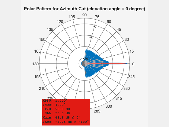
As NEXRAD is a polarimetric radar, modeling the polarimetric characteristics of the antenna is important. According to NEXRAD specifications, the antenna pattern has a beamwidth of about 1 degree and first sidelobe below -30 dB.
azang = -180:0.5:180;
elang = -90:0.5:90;
% We synthesize a pattern using isotropic antenna elements and tapering the
% amplitude distribution to make it follow NEXRAD specifications.
magpattern = load('NEXRAD_pattern.mat');
phasepattern = zeros(size(magpattern.pat));
% The polarimetric antenna is assumed to have ideally matched horizontal
% and vertical polarization pattern.
hPolAntenna = phased.CustomAntennaElement(...
    'SpecifyPolarizationPattern',true,'AzimuthAngles',azang,'ElevationAngles',elang,...
    'HorizontalMagnitudePattern',magpattern.pat,'VerticalMagnitudePattern',-inf(size(magpattern.pat)), ...
    'HorizontalPhasePattern',phasepattern,'VerticalPhasePattern',phasepattern);
vPolAntenna = phased.CustomAntennaElement(...
    'SpecifyPolarizationPattern',true,'AzimuthAngles',azang,'ElevationAngles',elang,...
    'HorizontalMagnitudePattern',-inf(size(magpattern.pat)), 'VerticalMagnitudePattern',magpattern.pat,...
    'HorizontalPhasePattern',phasepattern,'VerticalPhasePattern',phasepattern);
Plot the azimuth cut of the antenna pattern in horizontal polarization.
D = pattern(hPolAntenna,fc,azang,0);
P = polarpattern(azang,D,'TitleTop','Polar Pattern for Azimuth Cut (elevation angle = 0 degree)');
P.AntennaMetrics = 1;
removeAllCursors(P);
Associate the array with the radiator and collector for each polarization.
radiatorH = phased.Radiator(...
    'Sensor',hPolAntenna,'Polarization','Combined',...
    'OperatingFrequency',fc);
collectorH = phased.Collector(...
    'Sensor',hPolAntenna,'Polarization','Combined',...
    'OperatingFrequency',fc);
radiatorV = phased.Radiator(...
    'Sensor',vPolAntenna,'Polarization','Combined',...
    'OperatingFrequency',fc);
collectorV = phased.Collector(...
    'Sensor',vPolAntenna,'Polarization','Combined',...
    'OperatingFrequency',fc);
To simulate a polarimetric radarTransceiver, define radarTransceiver for each polarization.
xcvrHH = radarTransceiver('Waveform',waveform, ...
    'Transmitter',transmitter,'TransmitAntenna',radiatorH, ...
    'Receiver',receiver,'ReceiveAntenna',collectorH,...
    'MechanicalScanMode','Circular','MechanicalScanRate',0);
xcvrVV = radarTransceiver('Waveform',waveform, ...
    'Transmitter',transmitter,'TransmitAntenna',radiatorV, ...
    'Receiver',receiver,'ReceiveAntenna',collectorV,...
    'MechanicalScanMode','Circular','MechanicalScanRate',0);
Weather Target
Generally, weather radar data is categorized into three levels. Level-I data is raw time series I/Q data as input to the signal processor in the Radar Data Acquisition unit. Level-II data consists of the radar spectral moments (reflectivity, radial velocity, and spectrum width) and polarimetric variables (differential reflectivity, correlation coefficient, and differential phase) output from the signal processor. Level-III data is the output product data of the radar product generator, such as hydrometeor classification, storm total precipitation, and tornadic vortex signature.
In this example, Level-II data from KTLX NEXRAD radar at 04:33:45 UTC on May 19th, 2013 is used. This data comes from a convective precipitation that occurred in Oklahoma and is used to generate scattering matrix of weather targets. The data is available via FTP download. It represents a volume scan that includes a series of 360-degree sweeps of the antenna at predetermined elevation angles completed in a specified period of time. In the data file name KTLX20130519_043345_V06, KTLX refers to the radar site name, 20130519_043345 refers to the date and time when the data was collected, and V06 refers to the data format of version 6. In this simulation, the lowest elevation cut (0.5 degree) is extracted from the volume scan data as an example.
Read the Level-II data into the workspace. Store it in the nexrad structure array, which contains all the radar moments as well as an azimuth field that specifies the azimuth angle for each radial data point in the Cartesian coordinate system. For simplicity, load NEXRAD data that was transformed from a compressed file to a MAT-file and round azimuth to the nearest integer.
load NEXRAD_data.mat;
nexrad.azimuth = round(nexrad.azimuth);
Define an area of interest (AOI) in terms of azimuth and range in Cartesian coordinates.
az1 = 42;           % Starting azimuth angle (degree)
az2 = 48;           % Ending azimuth angle (degree)
rg1 = 20000;        % Starting range (m)
rg2 = 30000;        % Ending range (m)
blindRng = 2000;    % NEXRAD's blind range
b0 = blindRng/rangeRes;         % Number of range bins within the blind range
numAz = az2-az1+1;              % Number of azimuth angles in the AOI
numBins = (rg2-rg1)/rangeRes+1; % Number of range bins in each azimuth
% Select AOI data and store it in _nexrad_aoi_ structure array, which
% contains all the radar moments, as well as starting and ending azimuth
% and range indices.
nexrad_aoi = helperSelectAOI(nexrad,az1,az2,rg1,rg2,blindRng,rangeRes);
Weather Measurements Collection
To model weather target comprised of distributed volume scatterers, each radar resolution volume is regarded as an equivalent scattering center whose scattering matrix is updated between pulse to pulse. In this example, the Monte Carlo method is used to simulate the randomly scattered wave field and generate scattering matrix from the NEXRAD Level-II data.
% Preallocate datacube
rxh_aoi = complex(zeros(numBins,numPulses));    % H-pol 2D datacube
rxv_aoi = complex(zeros(numBins,numPulses));    % V-pol 2D datacube
iqhh = complex(zeros(numAz,numBins,numPulses)); % H-pol 3D datacube
iqvv = complex(zeros(numAz,numBins,numPulses)); % V-pol 3D datacube
rdrpos = [0;0;0];   % Radar position (m)
el = 0;             % Elevation of target plane relative to radar
simTime = 0;        % Simulation time
sceneAxes = eye(3); % Scenario axes
% Mechanical scanning
for ii = 1:numAz
    az = nexrad.azimuth(nexrad_aoi.r1+ii-1);   % current azimuth
    axes = azelaxes(wrapTo180(az),el);         % current axes
    % Preallocate target position and target poses
    tgtpos = zeros(3,numBins);
    tgtPoses = repmat(struct('Position',zeros(3,1),...
        'Signatures',{}),1,numBins);
    for jj = 1:numBins
        rpos = (nexrad_aoi.b1+jj-2)*rangeRes + blindRng;
        tpos = [rpos*cosd(el)*cosd(az);rpos*cosd(el)*sind(az);rpos*sind(el)];
        tgtpos(:,jj) = tpos;
    end
    % Calculate the target range
    [tgtrng,~] = rangeangle(tgtpos,rdrpos,axes);
    % Initial mechanical scan angle for each dwell time
    release(xcvrHH);
    xcvrHH.InitialMechanicalScanAngle = az;
    release(xcvrVV);
    xcvrVV.InitialMechanicalScanAngle = az;
    for mm = 1:numPulses
        randStream = RandStream('twister','Seed',0);
        for jj = 1:numBins
            % Update scattering matrix of weather target every PRT
            [shhpat,svvpat] = helperScatteringMatrix(lambda,nexrad_aoi.ZH(ii,jj),nexrad_aoi.Vr(ii,jj),...
                nexrad_aoi.SW(ii,jj),nexrad_aoi.ZDR(ii,jj),nexrad_aoi.Rhohv(ii,jj),nexrad_aoi.Phidp(ii,jj),simTime,randStream);
            tgtPoses(jj).Signatures = rcsSignature('EnablePolarization',true, ...
                'ShhPattern',shhpat*tgtrng(jj),...
                'SvvPattern',svvpat*tgtrng(jj));
            tgtPoses(jj).Position = tgtpos(:,jj);
        end
        % Step H-pol radarTransceiver
        rxh = xcvrHH(tgtPoses,simTime,sceneAxes);
        % Step V-pol radarTransceiver
        rxv = xcvrVV(tgtPoses,simTime,sceneAxes);
        % Matched filtering
        rxh = matchedfilter(rxh);
        rxv = matchedfilter(rxv);
        rxh = [rxh(matchingdelay+1:end);zeros(matchingdelay,1)];
        rxv = [rxv(matchingdelay+1:end);zeros(matchingdelay,1)];
        % Discard blind range data and select AOI data
        rxh_aoi(:,mm) = rxh(nexrad_aoi.b1+b0:nexrad_aoi.b2+b0);
        rxv_aoi(:,mm) = rxv(nexrad_aoi.b1+b0:nexrad_aoi.b2+b0);
        % Update simulation time
        simTime = simTime + 1/prf;
    end
    iqhh(ii,:,:) = rxh_aoi;
    iqvv(ii,:,:) = rxv_aoi;
end
Weather Radar Moment Estimation
Using pulse pair processing, calculate all the radar moments from estimates of correlations, including reflectivity, radial velocity, spectrum width, differential reflectivity, correlation coefficient, and differential phase.
azimuth = nexrad.azimuth(nexrad_aoi.r1:nexrad_aoi.r2);
range = (nexrad_aoi.b1-1:nexrad_aoi.b2-1)*rangeRes + blindRng;
for ii = 1:numAz
    for jj = 1:numBins
        moment0 = helperPulsePairProcessing(squeeze(iqhh(ii,jj,:)),squeeze(iqvv(ii,jj,:)),lambda,prf,range(jj));
        moment.ZH(ii,jj) = moment0.ZH;
        moment.Vr(ii,jj) = moment0.Vr;
        moment.SW(ii,jj) = moment0.SW;
        moment.ZDR(ii,jj) = moment0.ZDR;
        moment.Rhohv(ii,jj) = moment0.Rhohv;
        moment.Phidp(ii,jj) = moment0.Phidp;
    end
end
Simulation Result
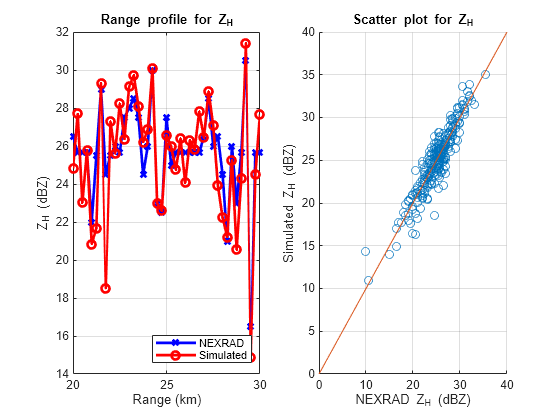
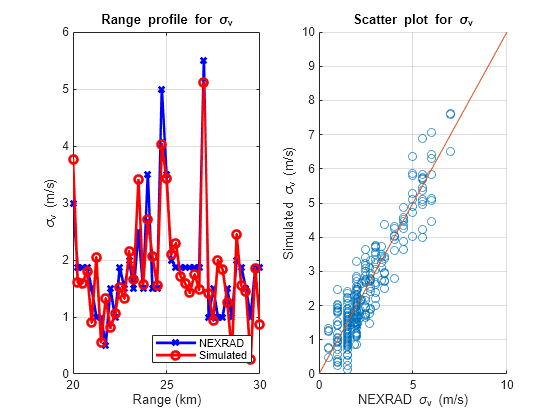
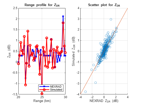
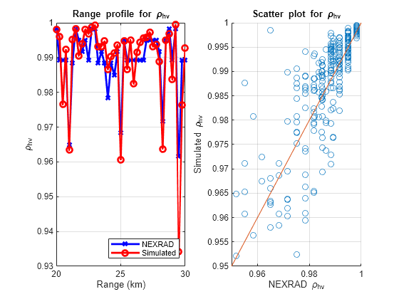
Compare the simulation result with the NEXRAD ground truth. Evaluate the simulated data quality using error statistics, a sector image, a range profile, and a scatter plot. Error statistics are expressed as the bias and standard deviation of the estimated radar moments compared to the NEXRAD Level-II data (truth fields).
Reflectivity
Reflectivity, , is the zeroth moment of the Doppler spectrum and is related to liquid water content or precipitation rate in the resolution volume. Because values of that are commonly encountered in weather observations span many orders of magnitude, radar meteorologists use a logarithmic scale given by as dBZ, where is in units of mm^6/m^3.
[ZHBias,ZHStd] = helperDataQuality(nexrad_aoi,moment,range,azimuth,'ZH');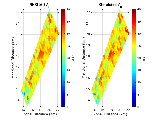
Radial Velocity
Radial velocity, , is the first moment of the power-normalized spectra, which reflects the air motion toward or away from the radar.
[VrBias,VrStd] = helperDataQuality(nexrad_aoi,moment,range,azimuth,'Vr');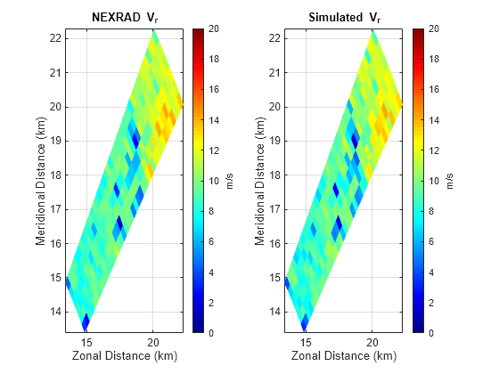

Spectrum Width
Spectrum width, , is the square root of the second moment of the normalized spectrum. The spectrum width is a measure of the velocity dispersion, that is, shear or turbulence within the resolution volume.
[SWBias,SWStd] = helperDataQuality(nexrad_aoi,moment,range,azimuth,'SW');
Differential Reflectivity
Differential reflectivity, , is estimated from the ratio of the returned power for the horizontal and vertical polarization signals. The differential reflectivity is useful in hydrometeor classification.
[ZDRBias,ZDRStd] = helperDataQuality(nexrad_aoi,moment,range,azimuth,'ZDR');
Correlation Coefficient
The correlation coefficient, , represents the consistency of the horizontal and vertical returned power and phase for each pulse. The correlation coefficient plays an important role in determining polarimetric radar system performance and classifying radar echo types.
[RhohvBias,RhohvStd] = helperDataQuality(nexrad_aoi,moment,range,azimuth,'Rhohv');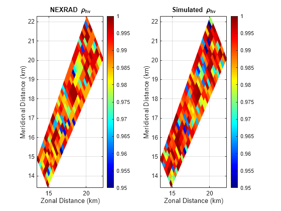
Differential Phase
The differential phase, , is the difference in the phase delay of the returned pulse between the horizontal and vertical polarizations. The differential phase provides information on the nature of the scatterers that are being sampled.
[PhidpBias,PhidpStd] = helperDataQuality(nexrad_aoi,moment,range,azimuth,'Phidp');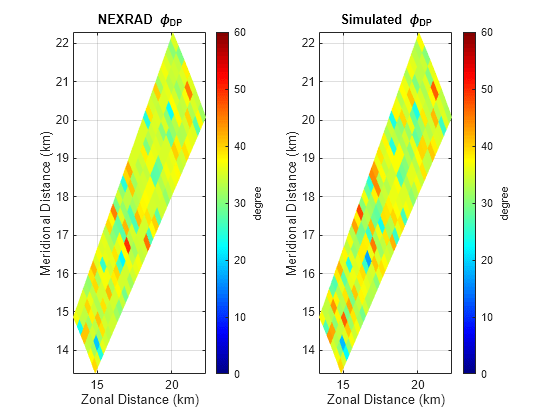

Error Statistics
Figures in previous sections provide a visual qualitative measure of the simulation quality. This section of the example shows the quantitative comparison of the estimates with NEXRAD ground truth as error statistics including bias and standard deviation (STD).
MomentName = {'ZH';'Vr';'SW';'ZDR';'Rhohv';'Phidp'};
BiasEstimate = [round(mean(ZHBias),2);round(mean(VrBias),2);round(mean(SWBias),2);...
    round(mean(ZDRBias),2);round(mean(RhohvBias),3);round(mean(PhidpBias),2)];
StdEstimate = [round(mean(ZHStd),2);round(mean(VrStd),2);round(mean(SWStd),2);...
    round(mean(ZDRStd),2);round(mean(RhohvStd),3);round(mean(PhidpStd),2)];
StdTruth = helperTruthSTD(nexrad_aoi.SW,nexrad_aoi.Rhohv,numPulses,1/prf,lambda);
StdTheory = [round(StdTruth.ZH,2);round(StdTruth.Vr,2);round(StdTruth.SW,2);...
    round(StdTruth.ZDR,2);round(StdTruth.Rhohv,3);round(StdTruth.Phidp,2)];
Unit = {'dB';'m/s';'m/s';'dB';'Unitless';'degree'};
T = table(MomentName,BiasEstimate,StdEstimate,StdTheory,Unit);
disp(T);
MomentName BiasEstimate StdEstimate StdTheory Unit
__________ ____________ ___________ _________ ____________
{'ZH' } 0 1.37 1.25 {'dB' }
{'Vr' } -0.09 0.57 0.48 {'m/s' }
{'SW' } -0.06 0.56 0.47 {'m/s' }
{'ZDR' } 0.03 0.36 0.32 {'dB' }
{'Rhohv'} 0.001 0.008 0.006 {'Unitless'}
{'Phidp'} 0.03 2.15 2.11 {'degree' }
By comparison, the mean bias for all the radar estimates is close to zero, and the STD of all the radar estimates is consistent with the STD of theory. It is expected that the STD of estimates is a little bit larger than the STD of theory because of sampling error. If numPulses is increased, the STD of estimates will be closer to the STD of theory, while it will take a longer time to run the simulation.
Summary
This example showed how to simulate the polarimetric Doppler radar returns from an area of distributed weather targets. Visual comparison and error statistics showed the estimated radar moments are consistent with NEXRAD ground truth. With this example, you can further explore the simulated time series data in other applications such as waveform design, clutter filtering, and data quality evaluation for weather radar.
References
[1] Doviak, R and D. Zrnic. Doppler Radar and Weather Observations, 2nd Ed. New York: Dover, 2006.
[2] Zhang, G. Weather Radar Polarimetry. Boca Raton: CRC Press, 2016.
[3] Li, Z, et al. "Polarimetric phased array weather radar data quality evaluation through combined analysis, simulation, and measurements," IEEE Geosci. Remote Sens. Lett., vol. 18, no. 6, pp. 1029–1033, Jun. 2021.


