5G 파형을 사용한 통합 센싱 및 통신
R2026b이 예제에서는 TR 38.901 ISAC 채널 모델을 사용하여 5G NR(New Radio) 파형의 ISAC(통합 센싱 및 통신) 기능을 보여줍니다. 5G NR 링크의 PDSCH(physical downlink shared channel)를 통해 데이터 프레임 송신을 시뮬레이션하고, 수신된 프레임에서 얻은 채널 행렬 추정값을 처리하여 채널에 존재하는 이동 UAV(무인 항공기) 센싱 타깃(ST)의 레이다 측정값을 추출하는 방법을 보여줍니다.
소개
ISAC의 핵심 개념은 동일한 하드웨어와 주파수 스펙트럼을 활용하여 통신과 센싱 기능을 동시에 수행하는 것입니다. 최근 연구에서는 새로운 이중 기능 시스템의 공동 설계부터 기존 무선 네트워크에서 센싱 기능을 구현하는 것까지 다양한 ISAC 접근 방식이 탐구되고 있습니다. 후자의 접근 방식은 기존 장비와 네트워크 인프라를 활용하므로 특히 매력적입니다. 센싱을 Beyond 5G(B5G) 및 6G와 같은 차세대 무선 네트워크에 통합하면 전자기 스펙트럼 혼잡을 완화하는 데 도움이 될 뿐만 아니라 새로운 다양한 응용이 가능해집니다. 여기에는 고정확도 위치추정 및 추적뿐만 아니라 사람의 행동 인식이 포함됩니다.
이 예제에서는 3GPP NR 표준에 정의된 5G NR 파형을 사용하여 이동 UAV 센싱 타깃을 효과적으로 센싱하는 방법을 보여줍니다. 수신된 PDSCH 프레임에서 얻은 채널 행렬 추정값은 송신 파형이 수신기로 전달되는 동안 발생하는 시간 지연과 도플러 편이에 대한 정보를 본질적으로 포함합니다. 이 정보를 표준 레이다 데이터 큐브 기법과 유사한 방식으로 처리함으로써, 이러한 시간 지연과 도플러 편이를 해당 UAV 센싱 타깃의 위치와 속도로 변환할 수 있으며, 이를 통해 레이다 검출이 이루어집니다.
이 예제는 먼저 단일 센싱 송신기(STX)와 단일 센싱 수신기(SRX)를 포함하는 ISAC-UAV 센싱 시나리오를 정의하는 것으로 시작합니다. TRP-UE 바이스태틱 센싱 모드를 적용하며, 여기서 STX는 기지국을 나타내고 SRX는 사용자 단말을 모델링합니다. 그런 후 송신 5G NR 파형을 구성하여 선택한 DM-RS(복조 기준 신호) 파라미터가 원하는 센싱 성능과 직접적으로 관련된다는 점을 보여줍니다. 다음으로 TR 38.901 ISAC 채널을 통한 PDSCH 프레임의 전파를 시뮬레이션합니다. 이 채널은 센싱 타깃과 배경 환경의 영향을 모두 받는 다중경로 성분을 모델링합니다. 수신된 각 프레임에 대해 채널 행렬을 추정 및 처리하여 채널에 존재하는 이동 UAV ST를 검출합니다.
이 예제는 센싱 관점에서 볼 때, 모델링된 5G 링크가 타깃의 바이스태틱 거리와 도래각을 측정할 수 있는 바이스태틱 레이다임을 보여줍니다. 마지막으로, 이러한 측정값을 추적 알고리즘에 전달하여 타깃 트랙을 구성하고 카테시안 좌표에서 타깃 위치와 속도를 추정합니다.
ISAC 시나리오
30GHz 주파수에서 동작하는 5G NR 링크가 있다고 가정해 보겠습니다.
rng('default');                                            % Set the random number generator for reproducibility
carrierFrequency = 30e9;                                   % Carrier frequency (Hz)
wavelength = freq2wavelen(carrierFrequency);
STX(gNodeB)는 높이 10미터에서 xy 평면의 원점에 위치하도록 구성합니다.
txPosition = [0; 0; 10]; % Base station locationSTX가 8개의 등방성 안테나 소자가 반파장 간격으로 배치된 균일 선형 배열(ULA)을 갖도록 구성합니다. 송신기 전력을 46dBm으로 설정합니다.
numTxAntennas = 8;                                         % Number of antenna elements at the Tx array
element = phased.IsotropicAntennaElement('BackBaffled', true);
txArray = phased.ULA(numTxAntennas, wavelength/2, 'Element', element);
txPower = 46;                                              % dBm
송신 배열의 법선이 x축 방향을 향하도록 설정합니다. txOrientation 벡터는 TR 38.901 Section 7.1.3에 지정된 대로 베어링(bearing), 다운틸트(downtilt), 경사(slant) 회전 각도를 각각 도 단위로 지정합니다.
txOrientation = [0; 0; 0]; % Tx array orientation [bearing; downtilt; slant] (degrees)SRX(사용자 단말)가 송신기에서 일정 거리 떨어져 위치하도록 구성합니다.
rxPosition = [50; 60; 2]; % User equipment locationSRX가 8개의 등방성 안테나 소자가 반파장 간격으로 배치된 균일 선형 배열(ULA)을 갖도록 구성합니다. 수신기 잡음 지수를 5dB로 설정합니다.
numRxAntennas = 8;                                         % Number of antenna elements at the Rx array
rxArray = phased.ULA(numRxAntennas, wavelength/2, 'Element', element);
rxNoiseFigure = 5;                                         % dB
수신 배열의 법선이 음의 y축 방향을 향하도록 설정합니다.
rxOrientation = [270; 0; 0]; % Rx array orientation [bearing; downtilt; slant] (degrees)helperGetTargetTrajectories 헬퍼 함수를 사용하여 2개의 이동 UAV 센싱 타깃에 대해 2개의 직선 등속 궤적을 생성합니다. 이들은 센싱 기능의 관심 타깃입니다.
targets.Trajectories = helperGetTargetTrajectories();
ans = 2×5 table
    Trajectory    Start Position [x, y, z]    End Position [x, y, z]    Length (m)    Speed (m/s)
    __________    ________________________    ______________________    __________    ___________

       "1"              {[25 -5 10]}               {[40 30 10]}           38.079        9.5197
       "2"              {[70 30 10]}               {[80 10 10]}           22.361        5.5902
numTargets = numel(targets.Trajectories);
h38901ISACChannel System object (TM) 객체를 사용하여 STX, ST, SRX 간 채널을 모델링합니다.
channel = h38901ISACChannel;

channel.SensingScenario = "ISAC-UAV";
channel.SensingMode = "TRP-UE Bistatic";
channel.CommunicationScenario = "UMi";

% Sensing Transmitter
channel.STX.Position = txPosition;
channel.STX.TransmitAntennaArray = txArray;
channel.STX.TransmitArrayOrientation = txOrientation;

% Sensing Receiver
channel.SRX.Position = rxPosition;
channel.SRX.ReceiveAntennaArray = rxArray;
channel.SRX.ReceiveArrayOrientation = rxOrientation;

% Sensing Targets
channel.STs = repmat(channel.STs,1,numTargets);
channel.STs(1) = applyInitialPose(channel.STs(1),targets.Trajectories{1});
channel.STs(2) = applyInitialPose(channel.STs(2),targets.Trajectories{2});

% Configure channel properties
channel.CenterFrequency = carrierFrequency;
channel.LOSProbability = 1;
channel.TargetPowerOffset = 15; % (dB) for power normalization
channel.Seed = 4;
channel.ScenarioExtents = helperGetScenarioExtents(channel,targets.Trajectories);
helperVisualizeScenario 헬퍼 함수를 사용하여 시나리오를 시각화합니다.
helperVisualizeScenario(channel,targets.Trajectories);
title('ISAC Scenario');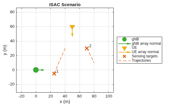
센싱 관점에서 보면 이 시나리오에서 송신기와 수신기는 바이스태틱 쌍을 이룹니다.
5G 파형 구성
5G NR에 대한 시스템 파라미터를 설정합니다. 채널 대역폭을 50MHz로 설정합니다.
channelBandwidth = 50; % Transmission bandwidth and guardbands (MHz)대역폭 점유율을 설정합니다. 이는 송신 대역폭과 채널 대역폭 간 비율입니다. 대역폭 점유율이 낮을수록 보호 대역의 크기가 증가하여 스펙트럼 방출이 감소하지만, 그 대가로 스펙트럼 효율이 떨어집니다.
bandwidthOccupancy = 0.9; % Ratio of transmission bandwidth to channel bandwidth부반송파 간격을 60kHz로 설정합니다.
subcarrierSpacing = 60; % Subcarrier spacing (kHz)helperGet5GWaveformConfiguration을 사용하여 5G 파형 구성을 생성합니다.
waveformConfig = helperGet5GWaveformConfiguration(channelBandwidth, bandwidthOccupancy, subcarrierSpacing);
waveformInfo = nrOFDMInfo(waveformConfig.Carrier)
waveformInfo = struct with fields:
                   Nfft: 1024
             SampleRate: 61440000
    CyclicPrefixLengths: [104 72 72 72 72 72 72 72 72 72 72 72 72 72 72 72 72 72 72 72 72 72 72 72 72 72 72 72 104 72 72 72 72 72 72 72 72 72 72 72 72 72 72 72 72 72 72 72 72 72 72 72 72 72 72 72]
          SymbolLengths: [1128 1096 1096 1096 1096 1096 1096 1096 1096 1096 1096 1096 1096 1096 1096 1096 1096 1096 1096 1096 1096 1096 1096 1096 1096 1096 1096 1096 1128 1096 1096 1096 1096 1096 1096 1096 1096 1096 1096 1096 1096 1096 … ] (1×56 double)
              Windowing: 36
           SymbolPhases: [0 0 0 0 0 0 0 0 0 0 0 0 0 0 0 0 0 0 0 0 0 0 0 0 0 0 0 0 0 0 0 0 0 0 0 0 0 0 0 0 0 0 0 0 0 0 0 0 0 0 0 0 0 0 0 0]
         SymbolsPerSlot: 14
       SlotsPerSubframe: 4
          SlotsPerFrame: 40
transmissionBandwidth = subcarrierSpacing*1e3*waveformConfig.Carrier.NSizeGrid*12; % Bandwidth of resource blocks (Hz)
fprintf("Transmission bandwidth: %.2f MHz\n",transmissionBandwidth*1e-6);
Transmission bandwidth: 44.64 MHz
채널 샘플 레이트를 파형 샘플 레이트와 동일하게 설정합니다.
channel.SampleRate = waveformInfo.SampleRate;
PDSCH 프레임은 수신기가 채널 특성을 추정하는 데 도움이 되는 DM-RS 신호를 포함합니다. 통신 기능은 이 정보를 사용하여 송신된 데이터를 올바르게 복조합니다. 센싱 기능은 동일한 정보를 사용하여 채널에 존재하는 센싱 타깃의 위치와 속도를 추정할 수 있습니다. DM-RS 파일럿 신호 구성은 센싱 성능에 직접적으로 영향을 미칩니다. 여러 DM-RS 구성에 대한 자세한 내용은 NR PDSCH Resource Allocation and DM-RS and PT-RS Reference Signals (5G Toolbox) 예제를 참조하십시오.
DM-RS 파라미터를 설정합니다.
waveformConfig.PDSCH.DMRS.DMRSTypeAPosition = 2;           % Mapping type A only. First DM-RS symbol position is 2
waveformConfig.PDSCH.DMRS.DMRSLength = 1;                  % Single-symbol DM-RS
waveformConfig.PDSCH.DMRS.DMRSAdditionalPosition = 2;      % Additional DM-RS symbol positions (max range 0...3)
waveformConfig.PDSCH.DMRS.NumCDMGroupsWithoutData = 1;     % Number of CDM groups without data
waveformConfig.PDSCH.DMRS.DMRSConfigurationType = 1;       % DM-RS configuration type (1,2)
구성된 리소스 그리드의 리소스 블록 하나를 시각화합니다.
resourceGrid = nrResourceGrid(waveformConfig.Carrier, waveformConfig.PDSCH.NumLayers);
ind = nrPDSCHDMRSIndices(waveformConfig.Carrier, waveformConfig.PDSCH);
resourceGrid(ind) = nrPDSCHDMRS(waveformConfig.Carrier, waveformConfig.PDSCH);

helperVisualizeResourceGrid(abs(resourceGrid(1:12,1:14,1)));
title({'PDSCH DM-RS Resource Elements in the Carrier Resource Grid', '(single resource block)'});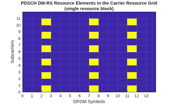
시간 영역에서 파일럿 신호의 밀도는 에일리어싱을 발생시키지 않으면서 모호성 없이 측정할 수 있는 최대 도플러 편이를 결정합니다. 구성된 PDSCH 프레임에서 시간 영역의 파일럿 신호 간 최대 간격은 = 5개 심볼입니다. 이에 대응되는 최대 비모호 도플러 편이(maximum unambiguous Doppler shift)는 다음 수식을 사용하여 계산할 수 있습니다.
여기서 은 심볼 지속 시간입니다.
% Compute maximum pilot signal separation in time
[~,pdschInfo] = nrPDSCHIndices(waveformConfig.Carrier,waveformConfig.PDSCH);
Mt = max(diff(pdschInfo.DMRSSymbolSet));

% Duration of an OFDM symbol in seconds
ofdmSymbolDuration = max(waveformInfo.SymbolLengths)/waveformInfo.SampleRate;

maxDoppler = 1/(2*Mt*ofdmSymbolDuration);
fprintf('Maximum unambiguous Doppler shift: %.2f kHz\n', maxDoppler*1e-3);
Maximum unambiguous Doppler shift: 5.45 kHz
이에 대응되는 최대 속도를 계산하고 이를 ISAC 시나리오의 타깃의 최대 대지 속도와 비교합니다.
maxVelocity = dop2speed(maxDoppler, wavelength)/2;
fprintf('Maximum unambiguous velocity: %.2f m/s\n', maxVelocity);
Maximum unambiguous velocity: 27.22 m/s
시나리오에 있는 타깃들의 속도가 최대 비모호 속도(maximum unambiguous velocity) 내에 있습니다.
마찬가지로, 주파수 영역에서 파일럿 신호의 밀도는 에일리어싱을 발생시키지 않으면서 측정할 수 있는 최대 시간 지연을 결정합니다. 주파수 영역에서 파일럿 신호는 = 2개 부반송파마다 반복됩니다. 이에 대응되는 최대 비모호 시간 지연(maximum unambiguous time delay)은 다음 수식을 사용하여 계산할 수 있습니다.
여기서 는 부반송파 간격입니다.
% Compute pilot signal separation in frequency
Mf = min(diff(waveformConfig.PDSCH.DMRS.DMRSSubcarrierLocations));
maxDelay = 1/(2*Mf*subcarrierSpacing*1e3);
fprintf('Maximum time delay: %.2fe-6 s\n', maxDelay*1e6);
Maximum time delay: 4.17e-6 s
이에 대응되는 최대 거리를 계산합니다.
% Baseline distance between Tx and Rx
baseline = vecnorm(txPosition - rxPosition);

% Propagation speed
propagationSpeed = physconst("LightSpeed");

% Bistatic maximum range
maxRange = maxDelay*propagationSpeed-baseline;
fprintf('Maximum unambiguous bistatic range: %.2f m\n', maxRange);
Maximum unambiguous bistatic range: 1170.62 m
시나리오에 있는 모든 타깃이 최대 비모호 거리(maximum unambiguous range) 내에 있습니다.
마지막으로, 송신 대역폭은 거리 분해능을 결정합니다.
% Range resolution
rangeResolution = propagationSpeed/transmissionBandwidth;
fprintf('Range resolution: %.2f m\n', rangeResolution);
Range resolution: 6.72 m
간격이 시스템의 거리 분해능보다 작고 도래각이 동일한 타깃들은 구분할 수 없습니다. 이 시나리오에서 두 관심 타깃은 거리와 각도 모두에서 잘 분리되어 있습니다.
채널 시뮬레이션 및 센싱 데이터 처리
이 예제에서는 10개의 PDSCH 프레임 송신을 시뮬레이션하며, 각 프레임은 0.4초 간격으로 송신되어 총 3.6초의 시간 길이를 포함합니다. 이러한 접근 방식은 타깃 위치의 변화를 효과적으로 보여주기 위해 필요합니다. 이 시간 구간 내의 모든 프레임을 시뮬레이션하는 것은 계산량이 너무 많아져서 현실적으로 수행하기 어렵습니다. 하지만, 시뮬레이션된 프레임 사이의 구간에서도 5G NR 링크가 정상적으로 동작한다고 가정합니다.
% Number of PDSCH frames to simulate
numSensingFrames = 10;

% Time step between simulated PDSCH frames (s)
dt = 0.4;

% Simulation times
t = (0:numSensingFrames-1)*dt;
채널 행렬 추정값은 각 PDSCH 프레임 송신에서 얻습니다. 채널 행렬은 차원 를 가지며, 여기서 는 부반송파 개수, 은 한 프레임에 포함된 OFDM 심볼의 총 개수, 은 수신 안테나 개수, 는 기준 신호 포트 개수입니다. 이 예제에서 기지국은 빔포밍을 수행하지 않으므로, 는 송신 안테나 개수와 같습니다. 채널 행렬 추정값은 레이다 데이터 큐브로 볼 수 있으며, 각 차원은 다음을 나타냅니다.
부반송파 차원: 거리(패스트 타임)
심볼 차원: 슬로우 타임
수신 안테나 차원: 도래각(AoA)
기준 신호 포트 차원: 발사각(AoD)
채널 행렬 추정값의 각 차원은 개별적으로 처리할 수 있습니다. 그런 다음 슬로우 타임 차원과 AoD 차원을 따라 비 코히어런스 방식으로 결과를 적분하여 거리-AoA 맵을 생성할 수 있으며, 이 맵을 타깃의 위치를 추정하는 데 사용할 수 있습니다.
이러한 처리를 수행하기 위해 AoA의 그리드를 정의하고 대응되는 조향 벡터를 계산합니다.
numAoA = ceil(2*pi*numRxAntennas);                         % AoA grid size
aoaGrid = linspace(-90, 90, numAoA);                       % AoA grid

% Receive array steering vectors
rxSteeringVector = phased.SteeringVector(SensorArray=channel.SRX.ReceiveAntennaArray);
rxsv = rxSteeringVector(carrierFrequency, aoaGrid);
AoD의 그리드를 정의하고 대응되는 조향 벡터를 계산합니다.
numAoD = ceil(2*pi*numTxAntennas);                         % AoD grid size
aodGrid = linspace(-90, 90, numAoD);                       % AoD grid

% Transmit array steering vectors
txSteeringVector = phased.SteeringVector(SensorArray=channel.STX.TransmitAntennaArray);
txsv = txSteeringVector(carrierFrequency, aodGrid);
바이스태틱 거리 그리드와 대응되는 패스트 타임 조향 벡터를 정의합니다.
% Limit the maximum bistatic range of interest to 100 meters
rangeGrid = -20:rangeResolution/4:100;                     % Bistatic range grid
numRange = numel(rangeGrid);                               % Bistatic range grid size

% Fast-time steering vectors
rangeFFTBins = (rangeGrid+baseline)/rangeResolution;
numSubcarriers = waveformConfig.Carrier.NSizeGrid*12;
k = (0:numSubcarriers-1).';
rngsv = (exp(2*pi*1i*k*rangeFFTBins/numSubcarriers)/numSubcarriers);
2차원 CFAR(일정 오경보율) 검출기를 설정하여 바이스태틱 거리-AoA 맵을 처리합니다. 거리 분해능과 각도 분해능을 기반으로 CFAR 보호 대역 크기를 결정합니다.
% Number of guard cells in range
numGuardCellsRange = ceil(rangeResolution/(rangeGrid(2)-rangeGrid(1))) + 1;

% Resolution in AoA domain
aoaResolution = ap2beamwidth((numRxAntennas-1)*channel.SRX.ReceiveAntennaArray.ElementSpacing, wavelength);

% Number of guard cells in AoA
numGuardCellsAoA = ceil(aoaResolution/(aoaGrid(2)-aoaGrid(1))) + 1;

% Create a 2-D CFAR detector
cfar2D = phased.CFARDetector2D('GuardBandSize',[numGuardCellsRange numGuardCellsAoA], 'TrainingBandSize', [4 6],...
    'ProbabilityFalseAlarm', 1e-3, 'OutputFormat', 'CUT result', 'ThresholdOutputPort', false);

% Compute indices of the cells under test
offsetIdxs = cfar2D.TrainingBandSize + cfar2D.GuardBandSize;

rangeIdxs = offsetIdxs(1)+1:numel(rangeGrid)-offsetIdxs(1);
angleIdxs = offsetIdxs(2)+1:numel(aoaGrid)-offsetIdxs(2);

[sumRangeIdxs, aoaIdxs] = meshgrid(rangeIdxs, angleIdxs);
cutidx = [sumRangeIdxs(:).'; aoaIdxs(:).'];
CFAR 알고리즘은 실제 타깃 위치 주변에서 여러 개의 검출 결과를 생성할 수 있습니다. 이러한 검출 결과들은 일반적으로 하나의 검출로 통합하기 위해 군집화됩니다. DBSCAN clusterer 객체를 생성합니다.
clusterer = clusterDBSCAN();
helperConfigureTracker 헬퍼 함수를 사용하여 타깃 추적 객체를 생성합니다. 반환된 추적기는 바이스태틱 거리 및 도래각 측정값을 사용해 추적을 수행하도록 구성되어 있습니다. 추적기의 상태 벡터는 카테시안 좌표로 표현합니다. 따라서 추적기는 타깃 위치 추정값을 개선할 뿐만 아니라 타깃 속도도 추정합니다.
% Define transmitter and receiver orientation axes
txOrientationAxes = rotationMatrix(txOrientation);
rxOrientationAxes = rotationMatrix(rxOrientation);

% Configure tracker
tracker = helperConfigureTracker(txPosition, rxPosition, txOrientationAxes, rxOrientationAxes, rangeResolution, aoaResolution);

% Preallocate space to store estimated target state vectors [x; vx; y; vy]
% Preallocate space for 10 tracks
targetStateEstimates = zeros(4, numSensingFrames, 10);
trackIDs = [];
ISAC 시나리오, 실제 타깃 위치, 타깃 검출 및 트랙을 함께 보여주는 시각화를 생성하기 위해 generateVisualizations를 true로 설정합니다.
% Produce visualizations generateVisualizations =false; if generateVisualizations scenarioCFARResultsFigure = figure; tl = tiledlayout(scenarioCFARResultsFigure, 1, 2, 'Padding', 'tight', 'TileSpacing', 'tight');
helperTheaterPlotter를 사용하여 시나리오, 타깃 궤적, 검출 및 트랙을 시각화합니다.
    scenarioPlotter = helperTheaterPlotter(tl);
    scenarioPlotter.plotTxAndRx(txPosition, rxPosition);
    scenarioPlotter.plotTrajectories(targets.Trajectories, t);
title(scenarioPlotter, 'ISAC Scenario');helperCFARResultsVisualizer를 사용하여 CFAR 결과를 시각화합니다.
    cfarResultsVisualizer = helperCFARResultsVisualizer(tl);
    xlabel(cfarResultsVisualizer, 'AoA (degrees)');
    ylabel(cfarResultsVisualizer, 'Bistatic Range (m)');
    title(cfarResultsVisualizer, 'CFAR Results');
end
한 번에 하나의 PDSCH 프레임을 송신하고 처리하는 시뮬레이션을 실행합니다.
% Number of symbols per frame
numSymbolsPerFrame = waveformInfo.SlotsPerFrame*waveformInfo.SymbolsPerSlot;

% Transmit and process one PDSCH frame at a time
for i = 1:numSensingFrames
    fprintf('\nSimulating frame at time %g s\n', t(i));

    % helperSimulateLinkSingleFrame returns a 4-D matrix
    % numSubcarriers x numSymbolsPerFrame x numRxAntennas x numTxAntennas
    sensingCSI = helperSimulateLinkSingleFrame(channel, waveformConfig, txPower, rxNoiseFigure, targets, t(i));

    % Process data cube by putting a zero in the first Doppler bin to filter out background noise
    X = fft(sensingCSI, [], 2);
    X(:, 1, :, :) = 0;
    x = ifft(X, [], 2);

    % Process data cube along the AoD dimension
    x = permute(x, [4 1 3 2]);
    x = txsv'*reshape(x, numTxAntennas, []);

    % Process data cube along the range dimension
    x = permute(reshape(x, numAoD, numSubcarriers, numRxAntennas, numSymbolsPerFrame), [2 3 1 4]);
    x = rngsv.'*reshape(x, numSubcarriers, []);

    % Process data cube along the AoA dimension
    x = permute(reshape(x, numRange, numRxAntennas, numAoD, numSymbolsPerFrame), [2 1 3 4]);
    x = rxsv'*reshape(x, numRxAntennas, []);

    % Average over AoDs and symbols
    x = reshape(x, numAoA, numRange, []);
    sumRangeAoAMap = sqrt(sum(abs(x).^2, 3)).';

    % Perform 2-D CFAR detection over range-AoA map
    cutResult = cfar2D(sumRangeAoAMap, cutidx);
    detectionIdxs = cutidx(:, cutResult);
    detectionValues = [rangeGrid(detectionIdxs(1,:)); aoaGrid(detectionIdxs(2,:))];

    % Cluster CFAR detections
    [~, clusterids] = clusterer(detectionValues.');
    uniqClusterIds = unique(clusterids);

    % Loop over detection clusters, and for each cluster find a
    % center
    m = numel(uniqClusterIds);
    clusteredDetections = zeros(2, m);

    for j = 1:m
        idxs = clusterids == uniqClusterIds(j);
        d = detectionValues(:, idxs);

        % Represent a cluster of detections with its center
        clusteredDetections(:, j) = mean(d, 2);
    end

    % Format detections so that they can be processed by the tracker
    detections = helperFormatDetectionsForTracker(clusteredDetections, t(i), rangeResolution, aoaResolution);

    % Pass detections to the tracker
    tracks = tracker(detections);

    % Store target state estimates
    for it = 1:numel(tracks)
        id = tracks(it).TrackID;
        trackIDs = union(trackIDs, id);
        targetStateEstimates(:, i, id) = tracks(it).State;
    end

    % Visualization
    if generateVisualizations
        % Plot true target positions
        targetPositions = zeros(numTargets, 3);
        for it = 1:numTargets
            targetPositions(it, :) = lookupPose(targets.Trajectories{it}, t(i));
        end
        scenarioPlotter.plotTargetPositions(targetPositions);

        % Plot target positions estimated from the detections
        measuredPositions = helperGetCartesianMeasurement(clusteredDetections, txPosition, rxPosition, rxOrientationAxes);
        scenarioPlotter.plotDetections(measuredPositions);
        scenarioPlotter.plotTracks(tracks);

        % Visualize CFAR results
        [trueRrx, trueAoA] = rangeangle(targetPositions.', rxPosition, rxOrientationAxes);
        [trueRtx, trueAoD] = rangeangle(targetPositions.', txPosition, txOrientationAxes);
        trueBistaticRange = trueRrx + trueRtx - baseline;

        cfarResultsVisualizer.plotCFARImage(aoaGrid, rangeGrid, sumRangeAoAMap);
        cfarResultsVisualizer.plotTruth([trueBistaticRange; trueAoA(1, :)]);
        cfarResultsVisualizer.plotClusteredDetections(clusteredDetections);

        sgtitle(scenarioCFARResultsFigure, sprintf('Frame %d, Simulation Time %.1f s', i, t(i)), 'FontSize' ,10);

        drawnow;
    end
end
Simulating frame at time 0 s
Throughput(Mbps) for 1 frame(s) = 1.7928
Throughput(%) for 1 frame(s) = 100.0000
Simulating frame at time 0.4 s
Throughput(Mbps) for 1 frame(s) = 1.7928
Throughput(%) for 1 frame(s) = 100.0000
Simulating frame at time 0.8 s
Throughput(Mbps) for 1 frame(s) = 1.7928
Throughput(%) for 1 frame(s) = 100.0000
Simulating frame at time 1.2 s
Throughput(Mbps) for 1 frame(s) = 1.7928
Throughput(%) for 1 frame(s) = 100.0000
Simulating frame at time 1.6 s
Throughput(Mbps) for 1 frame(s) = 1.7928
Throughput(%) for 1 frame(s) = 100.0000
Simulating frame at time 2 s
Throughput(Mbps) for 1 frame(s) = 1.7928
Throughput(%) for 1 frame(s) = 100.0000
Simulating frame at time 2.4 s
Throughput(Mbps) for 1 frame(s) = 1.7928
Throughput(%) for 1 frame(s) = 100.0000
Simulating frame at time 2.8 s
Throughput(Mbps) for 1 frame(s) = 1.7928
Throughput(%) for 1 frame(s) = 100.0000
Simulating frame at time 3.2 s
Throughput(Mbps) for 1 frame(s) = 1.7928
Throughput(%) for 1 frame(s) = 100.0000
Simulating frame at time 3.6 s
Throughput(Mbps) for 1 frame(s) = 1.7928
Throughput(%) for 1 frame(s) = 100.0000
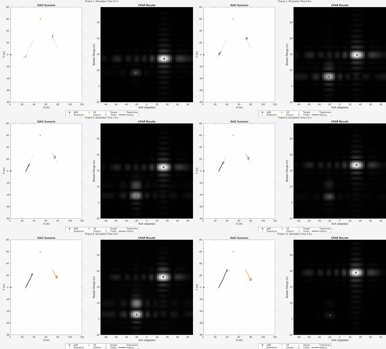
시뮬레이션 결과는 채널 행렬 추정값을 처리하여 바이스태틱 거리-AoA 공간에서 레이다 검출을 성공적으로 형성할 수 있음을 보여줍니다. 해당 검출 결과들은 실제 타깃 위치와 가깝습니다. 이후에 추적기는 이러한 검출을 활용하여 카테시안 좌표에서 위치와 속도로 구성된 타깃 상태를 추정합니다.
helperPlotSpeedEstimationResults 헬퍼 함수를 사용하여 추적기 출력값을 기반으로 한 타깃 속도 및 방향 추정값을 실제 값과 비교합니다.
helperPlotSpeedEstimationResults(t, targets.Trajectories, targetStateEstimates, trackIDs)
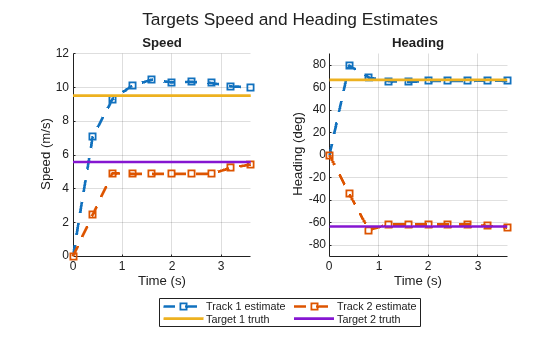
추적기가 추적을 시작하고 속도 계산을 시작하려면 적어도 2개의 초기 검출 결과가 필요합니다. 이러한 이유로 속도와 방향 추정값이 실제 값으로 수렴하기까지 여러 번의 트랙 업데이트가 필요할 수 있습니다.
결론
이 예제에서는 PDSCH 프레임을 송신하는 동안 얻은 채널 행렬 추정값에서 바이스태틱 레이다 정보를 추출하는 과정을 보여줌으로써 5G NR 파형의 센싱 기능을 설명합니다. 또한 선택한 DM-RS 파라미터가 센싱 성능에 미치는 영향을 설명합니다. 그런 다음 여러 개의 PDSCH 프레임이 송신되는 ISAC 시나리오를 시뮬레이션합니다. 수신된 각 프레임에 대해 채널 행렬은 레이다 데이터 큐브와 유사한 방식으로 처리됩니다. 이 예제는 바이스태틱 거리 및 AoA 추정을 위한 신호 처리 체인을 설정하는 방법을 보여줍니다. 이 처리 체인에는 거리 및 각도 응답 계산이 포함되며, 이어서 CFAR 검출 및 DBSCAN 군집화를 수행해 검출 결과를 생성합니다. 마지막으로, 바이스태틱 거리 및 AoA 공간에서 얻은 검출을 추적 알고리즘에 입력하여, 카테시안 좌표에서 타깃의 위치와 속도 추정값을 계산합니다.
지원 함수
function tracker = helperConfigureTracker(txPosition, rxPosition, txOrientationAxes, rxOrientationAxes, rangeResolution, aoaResolution)

    % Sensor specification
    sensorSpec = trackerSensorSpec("aerospace", "radar", "bistatic");
    sensorSpec.MeasurementMode = "range-angle";
    sensorSpec.IsReceiverStationary = true;
    sensorSpec.IsEmitterStationary = true;
    sensorSpec.HasElevation = false;
    sensorSpec.HasRangeRate = false;
    sensorSpec.MaxNumLooksPerUpdate = 1;
    sensorSpec.MaxNumMeasurementsPerUpdate = 10;
    sensorSpec.EmitterPlatformPosition = txPosition;
    sensorSpec.EmitterPlatformOrientation = txOrientationAxes.';
    sensorSpec.ReceiverPlatformPosition = rxPosition;
    sensorSpec.ReceiverPlatformOrientation = rxOrientationAxes.';
    sensorSpec.RangeResolution = rangeResolution;
    sensorSpec.AzimuthResolution = aoaResolution;
    sensorSpec.ReceiverFieldOfView = [360 180];
    sensorSpec.EmitterFieldOfView = [360 180];
    sensorSpec.ReceiverRangeLimits = [0 500];
    sensorSpec.EmitterRangeLimits = [0 500];
    sensorSpec.DetectionProbability = 0.9;

    % Target specification
    targetSpec = trackerTargetSpec('custom');
    targetSpec.StateTransitionModel = targetStateTransitionModel('constant-velocity');
    targetSpec.StateTransitionModel.NumMotionDimensions = 2;
    targetSpec.StateTransitionModel.VelocityVariance = 15^2/3*eye(2);
    targetSpec.StateTransitionModel.AccelerationVariance = 0.01^2/3*eye(2);

    tracker = multiSensorTargetTracker(targetSpec,sensorSpec,"jipda");
    tracker.ConfirmationExistenceProbability = 0.98;
    tracker.MaxMahalanobisDistance = 10;

end

function detections = helperFormatDetectionsForTracker(clusteredDetections, currentTime, rangeResoultion, aoaResolution)

    numDetections = size(clusteredDetections, 2);
    detections.ReceiverLookTime = currentTime;
    detections.ReceiverLookAzimuth = 0;
    detections.ReceiverLookElevation = 0;
    detections.EmitterLookAzimuth = 0;
    detections.EmitterLookElevation = 0;
    detections.DetectionTime = ones(1, numDetections) * currentTime;
    detections.Azimuth = clusteredDetections(2, :);
    detections.Range = clusteredDetections(1, :);

    % The measurement accuracy is proportional to the sensor resolution and
    % depends on the SNR.
    detections.AzimuthAccuracy = ones(1, numDetections) * aoaResolution/12;
    detections.RangeAccuracy = ones(1, numDetections) * rangeResoultion/8;

end

function meascart = helperGetCartesianMeasurement(dets, txPosition, rxPosition, rxOrientationAxes)

    if ~isempty(dets)
        n = size(dets, 2);
        meassph = zeros(3, n);
        meassph(1, :) = dets(2, :);
        meassph(3, :) = dets(1, :);

        meassph = local2globalcoord(meassph, 'ss', [0; 0; 0], rxOrientationAxes);
        meascart = bistaticposest(meassph(3, :), meassph(1:2, :), eps*ones(1, n), repmat([eps; eps], 1, n),...
            txPosition, rxPosition, 'RangeMeasurement', 'BistaticRange');
    else
        meascart = [];
    end

end

function trajectories = helperGetTargetTrajectories()

    % Target 1 start and end points (x,y,z)
    waypoints = [25 -5 10;
                 40 30 10];
    timeOfArrival = [0 4];
    traj1 = waypointTrajectory(waypoints,timeOfArrival);

    % Target 2 start and end points (x,y,z)
    waypoints = [70 30 10;
                 80 10 10];

    timeOfArrival = [0 4];
    traj2 = waypointTrajectory(waypoints,timeOfArrival);

    trajectories = {traj1, traj2};

    Trajectory = strings(numel(trajectories), 1);
    Speed = zeros(numel(trajectories), 1);
    Length = zeros(numel(trajectories), 1);
    Start = cell(numel(trajectories), 1);
    Stop = cell(numel(trajectories), 1);

    for i = 1:numel(trajectories)
        Trajectory(i) = i;
        Start{i} = trajectories{i}.Waypoints(1,:);
        Stop{i} = trajectories{i}.Waypoints(end,:);
        Length(i) = vecnorm(trajectories{i}.Waypoints(1, :) - trajectories{i}.Waypoints(end, :));
        Speed(i) = max(trajectories{i}.GroundSpeed);
    end

    table(Trajectory, Start, Stop, Length, Speed, 'VariableNames',...
        {'Trajectory', 'Start Position [x, y, z]', 'End Position [x, y, z]', 'Length (m)', 'Speed (m/s)'})

end

function extents = helperGetScenarioExtents(channel,trajectories)

    % Derive channel's scenario extents from target trajectories and STX/SRX positions
    wp = cell(1,numel(trajectories));
    for i = 1:numel(trajectories)
        wp{i} = trajectories{i}.Waypoints;
    end
    wp = cat(3,wp{:});

    txPos = channel.STX.Position;
    rxPos = channel.SRX.Position;

    X = [squeeze(wp(1,1,:));squeeze(wp(2,1,:));txPos(1);rxPos(1)];
    Y = [squeeze(wp(1,2,:));squeeze(wp(2,2,:));txPos(2);rxPos(2)];

    extentMargin = 1; % m
    minX = min(X) - extentMargin;
    minY = min(Y) - extentMargin;
    width = max(X) - minX + extentMargin;
    height = max(Y) - minY + extentMargin;

    extents = [minX minY width height];

end

function helperPlotSpeedEstimationResults(t, trajectories, targetStateEstimates, trackIDs)

    fig = figure;
    tl = tiledlayout(fig, 1, 2);
    speedAxes = nexttile(tl);
    hold(speedAxes, 'on');

    xlabel(speedAxes, 'Time (s)');
    ylabel(speedAxes, 'Speed (m/s)');
    grid(speedAxes, 'on');
    title(speedAxes, 'Speed');
    xlim(speedAxes, [t(1) t(end)]);
    lgd = legend(speedAxes, 'Location', 'southeast', 'Orientation', 'horizontal', 'NumColumns', 2);
    lgd.Layout.Tile = 'south';

    headingAxes = nexttile(tl);
    hold(headingAxes, 'on');
    xlabel(headingAxes, 'Time (s)');
    ylabel(headingAxes, 'Heading (deg)');
    grid(headingAxes, 'on');
    title(headingAxes, 'Heading');
    ylim(headingAxes, [-90 90]);
    xlim(headingAxes, [t(1) t(end)]);

    sgtitle(fig, 'Targets Speed and Heading Estimates')

    for it = 1:numel(trackIDs)
        id = trackIDs(it);
        vx = targetStateEstimates(2, :, id);
        vy = targetStateEstimates(4, :, id);

        speedEstimate = sqrt(vx.^2 + vy.^2);
        headingEstimate = atan2d(vy, vx);
        plot(speedAxes, t, speedEstimate, 's--', 'LineWidth', 2, 'DisplayName', sprintf('Track %d estimate', trackIDs(it)));
        plot(headingAxes, t, headingEstimate, 's--', 'LineWidth', 2);
    end

    for it = 1:numel(trajectories)
        [~, ~, velocity] = lookupPose(trajectories{it}, t);
        trueSpeed = sqrt(velocity(:, 1).^2 + velocity(:, 2).^2);
        trueHeading = atan2d(velocity(:, 2), velocity(:, 1));

        plot(speedAxes, t, trueSpeed, '-', 'LineWidth', 2, 'DisplayName', sprintf('Target %d truth', it));
        plot(headingAxes, t, trueHeading, '-', 'LineWidth', 2);
    end

end

function R = rotationMatrix(angles)

    % Determine the "ZYX" axis-sequence rotation matrix from the set of
    % bearing, downtilt, and slant angles specifying the array orientation
    R = rotz(angles(1))*roty(angles(2))*rotx(angles(3));

end

function ST = applyInitialPose(ST,trajectory)

    ST.Position = trajectory.Waypoints(1,:);
    ST.Orientation = [0 0 0];
    ST.Velocity = trajectory.Velocities(1,:);

end

