plotResponse
System object: phased.RangeResponse
Namespace: phased
Plot range response
Syntax
Description
plotResponse(
plots the range response with additional options specified by one or more
response,___,Name=Value)Name=Value pair arguments.
Input Arguments
Name-Value Arguments
Examples
Plot the radar range response of three targets using the plotResponse method of the phased.RangeResponse System object™. The transmitter and receiver are collocated isotropic antenna elements forming a monostatic radar system. The transmitted signal is a linear FM waveform with a pulse repetition interval of 7.0 μs and a duty cycle of 2%. The operating frequency is 77 GHz and the sample rate is 150 MHz.
fs = 150e6;fs = 150e6;
c = physconst("LightSpeed");
fc = 77e9;
pri = 7e-6;
prf = 1/pri;
Set up the scenario parameters. The radar transmitter and receiver are stationary and located at the origin. The targets are 500, 530, and 750 meters from the radars on the x-axis. The targets move along the x-axis at speeds of −60, 20, and 40 m/s. All three targets have a nonfluctuating RCS of 10 dB.
Create the target and radar platforms.
Numtgts = 3;
tgtpos = zeros(Numtgts);
tgtpos(1,:) = [500 530 750];
tgtvel = zeros(3,Numtgts);
tgtvel(1,:) = [-60 20 40];
tgtrcs = db2pow(10)*[1 1 1];
tgtmotion = phased.Platform(tgtpos,tgtvel);
target = phased.RadarTarget(PropagationSpeed=c,OperatingFrequency=fc, ...
    MeanRCS=tgtrcs);
radarpos = [0;0;0];
radarvel = [0;0;0];
radarmotion = phased.Platform(radarpos,radarvel);
Create the transmitter and receiver antennas.
txantenna = phased.IsotropicAntennaElement;
rxantenna = clone(txantenna);
Set up the transmitter-end signal processing. Construct an upsweep linear FM signal with a bandwidth of half the sample rate. Find the rms bandwidth and rms range resolution.
bw = fs/2;
waveform = phased.LinearFMWaveform(SampleRate=fs,...
    PRF=prf,OutputFormat="Pulses",NumPulses=1,SweepBandwidth=fs/2,...
    DurationSpecification="Duty cycle",DutyCycle=.02);
sig = waveform();
Nr = length(sig);
bwrms = bandwidth(waveform)/sqrt(12);
rngrms = c/bwrms;
Set up the transmitter and radiator System object properties. The peak output power is 10 W and the transmitter gain is 36 dB.
peakpower = 10;
txgain = 36.0;
transmitter = phased.Transmitter(...
    PeakPower=peakpower,...
    Gain=txgain,...
    InUseOutputPort=true);
radiator = phased.Radiator(...
    Sensor=txantenna,...
    PropagationSpeed=c,...
    OperatingFrequency=fc);
Create a free-space propagation channel in two-way propagation mode.
channel = phased.FreeSpace(...
    SampleRate=fs,...
    PropagationSpeed=c,...
    OperatingFrequency=fc,...
    TwoWayPropagation=true);
Set up the receiver-end processing. The receiver gain is 42 dB and noise figure is 10.
collector = phased.Collector(...
    Sensor=rxantenna,...
    PropagationSpeed=c,...
    OperatingFrequency=fc);
rxgain = 42.0;
noisefig = 10;
receiver = phased.ReceiverPreamp(...
    SampleRate=fs,...
    Gain=rxgain,...
    NoiseFigure=noisefig);
Loop over 128 pulses to build a data cube. For each step of the loop, move the target and propagate the signal. Then put the received signal into the data cube. The data cube contains the received signal per pulse. Ordinarily, a data cube has three dimensions. The last dimension corresponds to antennas or beams. Because only one sensor is used in this example, the cube has only two dimensions.
The processing steps are:
Move the radar and targets.
Transmit a waveform.
Propagate the waveform signal to the target.
Reflect the signal from the target.
Propagate the waveform back to the radar. Two-way propagation mode allows the return propagation to be combined with the outbound propagation.
Receive the signal at the radar.
Load the signal into the data cube.
Np = 128;
cube = zeros(Nr,Np);
for n = 1:Np
    [sensorpos,sensorvel] = radarmotion(pri);
    [tgtpos,tgtvel] = tgtmotion(pri);
    [tgtrng,tgtang] = rangeangle(tgtpos,sensorpos);
    sig = waveform();
    [txsig,txstatus] = transmitter(sig);
    txsig = radiator(txsig,tgtang);
    txsig = channel(txsig,sensorpos,tgtpos,sensorvel,tgtvel);
    tgtsig = target(txsig);
    rxcol = collector(tgtsig,tgtang);
    rxsig = receiver(rxcol);
    cube(:,n) = rxsig;
end
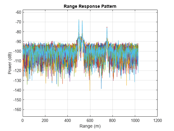
Create a phased.RangeResponse System object in matched filter mode. Then, call the plotResponse method to show the first 20 pulses.
matchcoeff = getMatchedFilter(waveform);
rangeresp = phased.RangeResponse(SampleRate=fs,PropagationSpeed=c);
plotResponse(rangeresp,cube(:,1:20),matchcoeff);
Version History
Introduced in R2017a