Structural Dynamics of Tuning Fork
This example shows how to perform modal and transient analysis of a tuning fork.
A tuning fork is a U-shaped beam. When struck on one of its prongs or tines, it vibrates at its fundamental (first) frequency and produces an audible sound.
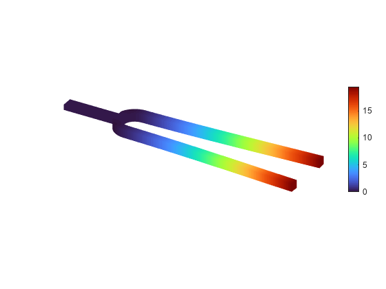
The first flexible mode of a tuning fork is characterized by symmetric vibration of the tines: they move towards and away from each other simultaneously, balancing the forces at the base where they intersect. The fundamental mode of vibration does not produce any bending effect on the handle attached at the intersection of the tines. The lack of bending at the base enables easy handling of the tuning fork without influencing its dynamics.
Transverse vibration of the tines causes the handle to vibrate axially at the fundamental frequency. This axial vibration can be used to amplify the audible sound by bringing the end of the handle in contact with a larger surface area, like a metal table top. The next higher mode with a symmetric mode shape is about 6.25 times the fundamental frequency. Therefore, a properly excited tuning fork vibrates with a dominant frequency corresponding to the fundamental frequency, producing a pure audible tone. This example simulates these aspects of the tuning fork dynamics by performing a modal analysis and a transient dynamics simulation.
You can find the helper functions animateSixTuningForkModes and tuningForkFFT and the geometry file TuningFork.stl at matlab/R20XXx/examples/pde/main.
Modal Analysis of Tuning Fork
Find natural frequencies and mode shapes for the fundamental mode and the next several modes of a tuning fork. Show the lack of bending effect on the fork handle at the fundamental frequency.
First, create a finite element model for modal analysis of a solid tuning fork.
model = femodel(AnalysisType="structuralModal", ...
                Geometry="TuningFork.stl");
Plot the tuning fork geometry.
pdegplot(model);

To perform unconstrained modal analysis of a structure, it is enough to specify the geometry, mesh, and material properties. First, specify Young's modulus, Poisson's ratio, and the mass density to model linear elastic material behavior. Specify all physical properties in consistent units.
E = 210e9;
nu = 0.3;
rho = 8000;
model.MaterialProperties = materialProperties(YoungsModulus=E, ...
                                              PoissonsRatio=nu, ...
                                              MassDensity=rho);
Generate a mesh.
model = generateMesh(model,Hmax=0.001);
Solve the model for a chosen frequency range. Specify the lower frequency limit below zero so that all modes with frequencies near zero appear in the solution.
RF = solve(model,FrequencyRange=[-Inf,4000]*2*pi);
By default, the solver returns circular frequencies.
modeID = 1:numel(RF.NaturalFrequencies);
Express the resulting frequencies in Hz by dividing them by . Display the frequencies in a table.
tmodalResults = table(modeID.',RF.NaturalFrequencies/(2*pi));
tmodalResults.Properties.VariableNames = {'Mode','Frequency'};
disp(tmodalResults);
Mode Frequency
____ _________
1 0.008488
2 0.0082989
3 0.0060921
4 0.0057719
5 0.0049471
6 0.0027135
7 460.42
8 706.29
9 1911.5
10 2105.6
11 2906.6
12 3814.6
Because there are no boundary constraints in this example, modal results include the rigid body modes. The first six near-zero frequencies indicate the six rigid body modes of a 3-D solid body. The first flexible mode is the seventh mode with a frequency around 460 Hz.
The best way to visualize mode shapes is to animate the harmonic motion at their respective frequencies. You can use the Visualize PDE Results Live Editor task to animate the data. Specify the results to visualize as RF and the type as Mode shapes. Specify the mode as the first flexible mode (the seventh mode in the list) and select Animate.
% Data to visualize
meshData = RF.Mesh;
nodalData = RF.ModeShapes.Magnitude(:,7);
deformationData = [RF.ModeShapes.ux(:,7) ...
    RF.ModeShapes.uy(:,7) ...
    RF.ModeShapes.uz(:,7)];
phaseData = cospi(0) + 1i*sinpi(0);

% Create PDE result visualization
resultViz = pdeviz(meshData,abs(real(nodalData*phaseData)), ...
    "DeformationData",deformationData*phaseData, ...
    "DeformationScaleFactor",0.00016521, ...
    "AxesVisible",false, ...
    "ColorbarVisible",false, ...
    "ColorLimits",[0 19.48]);

% Fix axes limits for animation
resultViz.XLimits = [-0.00023778 0.090685];
resultViz.YLimits = [-0.00021773 0.014618];
resultViz.ZLimits = [-0.0029436 0.0059436];

% Animate
for ii = 0:0.01:2
    phaseData = cospi(ii) + 1i*sinpi(ii);
    resultViz.NodalData = abs(real(nodalData*phaseData));
    resultViz.DeformationData = deformationData*phaseData;
    pause(0.01)
end
% Clear temporary variables
clearvars meshData nodalData deformationData phaseData ii
Alternatively, you can programmatically animate the results. The animateSixTuningForkModes function animates the six flexible modes, which are modes 7 through 12 in the modal results RF.
frames = animateSixTuningForkModes(RF);
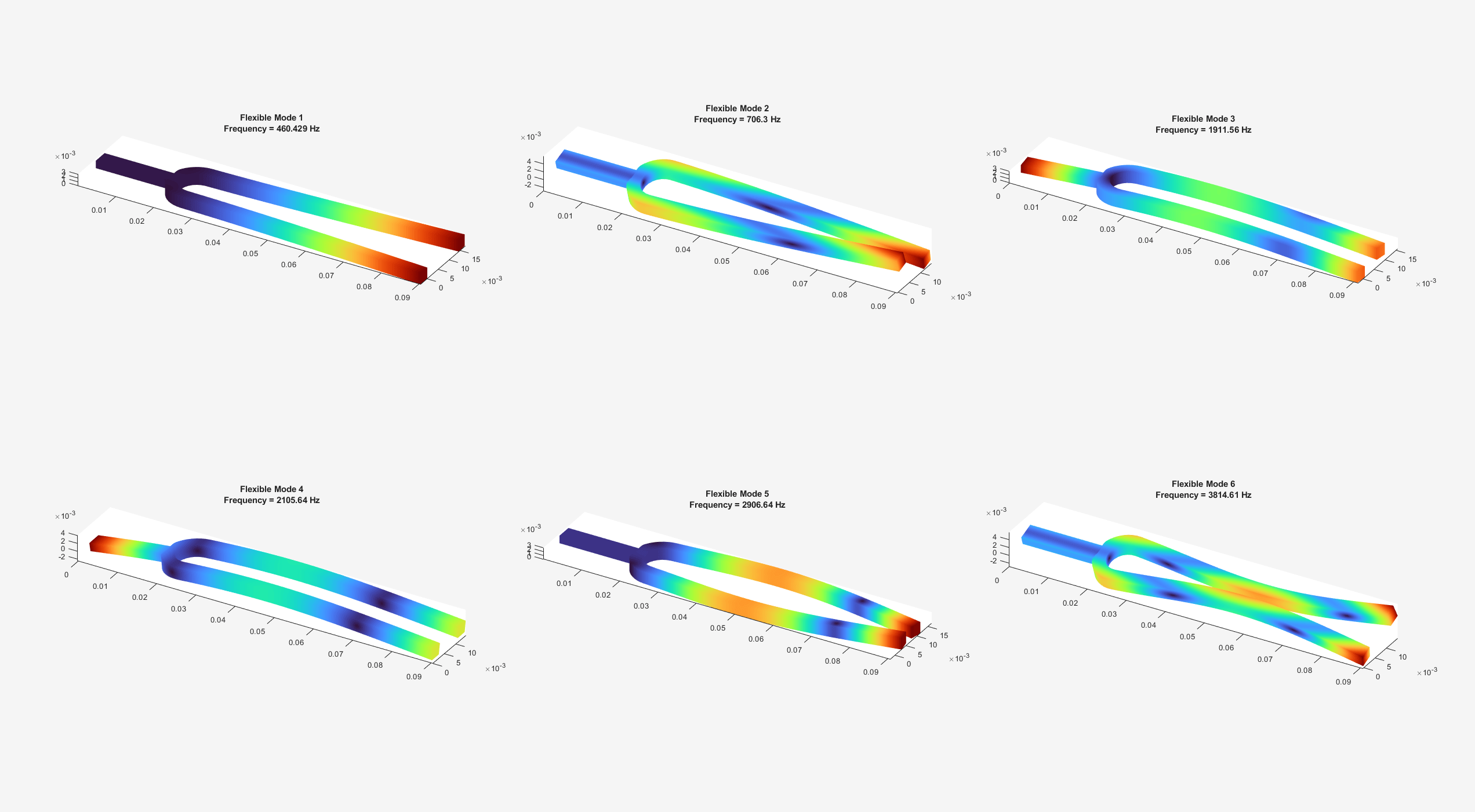
To play the animation, first create a figure window as follows:
h = figure;
h.Units="normalized";
h.OuterPosition=[0 0 1 1];
ax = gca;
ax.Visible=``"off";
Now use the movie command to play the animation.
movie(frames,5,30)
In the first mode, the two oscillating tines of the tuning fork balance out transverse forces at the handle. The next mode with this effect is the fifth flexible mode with the frequency around 2907 Hz. This frequency is about 6 times greater than the fundamental frequency of 460 Hz.
Transient Analysis of Tuning Fork
Simulate the dynamics of a tuning fork being gently and quickly struck on one of its tines. Analyze the vibration of the tines over time and the axial vibration of the handle.
First, switch the analysis type for the model object to transient structural.
model.AnalysisType = "structuralTransient";Generate a coarser mesh to speed up computations. Specify the Hface name-value argument to generate a finer mesh for small faces.
model = generateMesh(model,Hmax=0.005,Hface={[3 4 9 10],0.0003});Identify faces for applying boundary constraints and loads by plotting the geometry with the face labels.
figure("units","normalized","outerposition",[0 0 1 1])
pdegplot(model,FaceLabels="on");
view(-50,15)
title("Geometry with Face Labels")
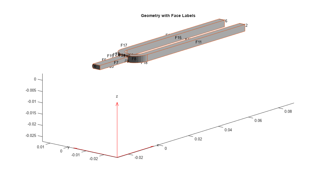
Impose sufficient boundary constraints to prevent rigid body motion under applied loading. Typically, you hold a tuning fork by hand or mount it on a table. A simplified approximation to this boundary condition is fixing a region near the intersection of the tines and the handle (faces 21 and 22).
model.FaceBC([21,22]) = faceBC(Constraint="fixed");Approximate an impulse loading on a face of a tine by applying a pressure load for a very small fraction of the time period of the fundamental mode. By using this very short pressure pulse, you ensure that only the fundamental mode of a tuning fork is excited. To evaluate the time period T of the fundamental mode, use the results of the modal analysis.
T7 = 2*pi/RF.NaturalFrequencies(7);
Specify the pressure loading on a tine as a short rectangular pressure pulse by using the trapezoidalLoad function. For details, see Trapezoidal Pulse Load.
P = 5e6;
T = setUpTrapezoid(EndTime=T7/300);
pressurePulse = @(location,state) trapezoidalLoad(P,location,state,T);
model.FaceLoad(11) = faceLoad(Pressure=pressurePulse);
Apply zero displacement and velocity as initial conditions.
model.CellIC = cellIC(Displacement=[0;0;0],Velocity=[0;0;0]);
Solve the transient model for 50 periods of the fundamental mode. Sample the dynamics 60 times per period of the fundamental mode.
ncycle = 50;
samplingFrequency = 60/T7;
tlist = linspace(0,ncycle*T7,ncycle*T7*samplingFrequency);
R = solve(model,tlist);
Plot the time-series of the vibration of the tine tip, which is face 12. Find nodes on the tip face and plot the y-component of the displacement over time using one of these nodes.
excitedTineTipNodes = findNodes(model.Geometry.Mesh,"region",Face=12);
tipDisp = R.Displacement.uy(excitedTineTipNodes(1),:);

figure
plot(R.SolutionTimes,tipDisp)
title("Transverse Displacement at Tine Tip")
xlim([0,0.1])
xlabel("Time")
ylabel("y-Displacement")
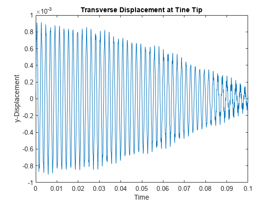
Perform a fast Fourier transform (FFT) of the tip displacement time-series to see that the vibration frequency of the tuning fork is close to its fundamental frequency. A small deviation from the fundamental frequency computed in an unconstrained modal analysis appears because of constraints imposed in the transient analysis.
[fTip,PTip] = tuningForkFFT(tipDisp,samplingFrequency);
figure
plot(fTip,PTip)
title(["Single-Sided Amplitude Spectrum","of Tip Vibration"])
xlabel("f (Hz)")
ylabel("|P1(f)|")
xlim([0,4000])

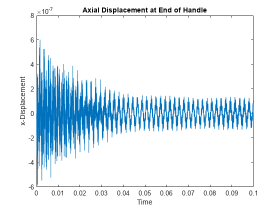
Transverse vibration of the tines causes the handle to vibrate axially with the same frequency. To observe this vibration, plot the axial displacement time-series of the end face of the handle.
baseNodes = model.Mesh.findNodes("region",Face=6);
baseDisp = R.Displacement.ux(baseNodes(1),:);
figure
plot(R.SolutionTimes,baseDisp)
title("Axial Displacement at End of Handle")
xlim([0,0.1])
ylabel("x-Displacement")
xlabel("Time")
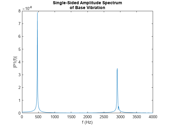
Perform an FFT of the time-series of the axial vibration of the handle. This vibration frequency is also close to its fundamental frequency.
[fBase,PBase] = tuningForkFFT(baseDisp,samplingFrequency);
figure
plot(fBase,PBase)
title(["Single-Sided Amplitude Spectrum","of Base Vibration"])
xlabel("f (Hz)")
ylabel("|P1(f)|")
xlim([0,4000])
Trapezoidal Pulse Load
Define a trapezoidal pulse function, trapezoidalLoad, to model rectangular, triangular, and trapezoidal load pulses. This function accepts the load magnitude, the location and state structure arrays, and the function specifying the pulse parameters that define the start, rise, fall, and end times.
function Tn = trapezoidalLoad(load,location,state,T)
if isnan(state.time)
    Tn = NaN*(location.nx);
    return
end
if isa(load,"function_handle")
    load = load(location,state);
else
    load = load(:);
end
% Four time-points that define a trapezoidal pulse
T1 = T(1); % Start time
T2 = T(2); % Rise time
T3 = T(3); % Fall time
T4 = T(4); % End time

% Determine multiplicative factor for the specified time
TnTrap = max([ ...
    min([(state.time - T1)/(T2-T1), ...
    1, ...
    (T4 - state.time)/(T4-T3)]), ...
    0]);
Tn = load.* TnTrap;
end
You can model rectangular, triangular, and trapezoidal load pulses.
For a rectangular pulse, specify the start and end times.
For a triangular pulse, specify the start time and any two of these times: rise time, fall time, and end time. You also can specify all four times, but they must be consistent.
For a trapezoidal pulse, specify all four times.

The setUpTrapezoid helper function accepts the name-value arguments StartTime, RiseTime, FallTime, and EndTime and processes these parameters for use in the trapezoidalLoad function. Pass the output of this function as the last argument of trapezoidalLoad. The default StartTime, RiseTime, and FallTime values are 0, while the default EndTime value is Inf.
function T = setUpTrapezoid(opts)
arguments
    opts.StartTime double {mustBeScalarOrEmpty,mustBeReal} = []
    opts.RiseTime  double {mustBeScalarOrEmpty,mustBeReal} = []
    opts.FallTime  double {mustBeScalarOrEmpty,mustBeReal} = []
    opts.EndTime   double {mustBeScalarOrEmpty,mustBeReal} = []
end
if isempty(opts.StartTime)
    opts.StartTime = 0;
end
if isempty(opts.RiseTime)
    opts.RiseTime = 0;
end
if isempty(opts.FallTime)
    opts.FallTime = 0;
end
if isempty(opts.EndTime) && (opts.FallTime ~= 0)
    opts.EndTime = opts.StartTime + opts.RiseTime + opts.FallTime;
elseif isempty(opts.EndTime) && (opts.FallTime == 0)
    opts.EndTime = Inf;
end
T = [opts.StartTime;
     opts.StartTime + opts.RiseTime;
     opts.EndTime - opts.FallTime;
     opts.EndTime];
end