electromagneticBC

Apply boundary conditions to electromagnetic model

Since R2021a

Domain-specific electromagnetic workflow is not recommended. New features might not be compatible with this workflow. For help migrating your existing code to the unified finite element workflow, see Migration from Domain-Specific to Unified Workflow.

Syntax

electromagneticBC(emagmodel,RegionType,RegionID,"Voltage",V)

electromagneticBC(emagmodel,RegionType,RegionID,"MagneticPotential",A)

electromagneticBC(emagmodel,RegionType,RegionID,"SurfaceCurrentDensity",K)

electromagneticBC(emagmodel,RegionType,RegionID,"ElectricField",E)

electromagneticBC(emagmodel,RegionType,RegionID,"MagneticField",H)

electromagneticBC(emagmodel,RegionType,RegionID,"FarField","absorbing","Thickness",h)

electromagneticBC(emagmodel,RegionType,RegionID,"FarField","absorbing","Thickness",h,"Exponent",e,"Scaling",s)

electromagneticBC(___,"Vectorized","on")

emagBC = electromagneticBC(___)

Description

electromagneticBC(emagmodel,RegionType,RegionID,"Voltage",V) adds a voltage boundary condition to emagmodel. The boundary condition applies to regions of type RegionType with ID numbers in RegionID. The solver uses a voltage boundary condition for an electrostatic analysis.

electromagneticBC(emagmodel,RegionType,RegionID,"MagneticPotential",A) adds a magnetic potential boundary condition to emagmodel. The solver uses a magnetic potential boundary condition for a magnetostatic analysis.

electromagneticBC(emagmodel,RegionType,RegionID,"SurfaceCurrentDensity",K) adds a surface current density boundary condition to emagmodel. The solver uses a surface current density boundary condition for a DC conduction analysis.

electromagneticBC(emagmodel,RegionType,RegionID,"ElectricField",E) adds an electric field boundary condition to emagmodel. The solver uses an electric field boundary condition for a harmonic analysis with the electric field type.

electromagneticBC(emagmodel,RegionType,RegionID,"MagneticField",H) adds a magnetic field boundary condition to emagmodel. The solver uses a magnetic field boundary condition for a harmonic analysis with the magnetic field type.

electromagneticBC(emagmodel,RegionType,RegionID,"FarField","absorbing","Thickness",h) adds an absorbing boundary condition to emagmodel and specifies the thickness of the absorbing region. The solver uses an absorbing boundary condition for a harmonic analysis.

electromagneticBC(emagmodel,RegionType,RegionID,"FarField","absorbing","Thickness",h,"Exponent",e,"Scaling",s) specifies the rate of attenuation of the waves entering the absorbing region. You can specify e, s, or both.

electromagneticBC(___,"Vectorized","on") uses vectorized function evaluation when you pass a function handle as an argument. If your function handle computes in a vectorized fashion, then using this argument saves time. For details on this evaluation, see More About and Vectorization.

Use this syntax with any of the input argument combinations in the previous syntaxes.

emagBC = electromagneticBC(___) returns the electromagnetic boundary condition object.

Examples

Specify Voltage on Boundaries

Create an electromagnetic model for electrostatic analysis.

emagmodel = createpde("electromagnetic","electrostatic");

Import and plot a geometry representing a plate with a hole.

gm = importGeometry(emagmodel,"PlateHoleSolid.stl");
pdegplot(gm,"FaceLabels","on","FaceAlpha",0.3)

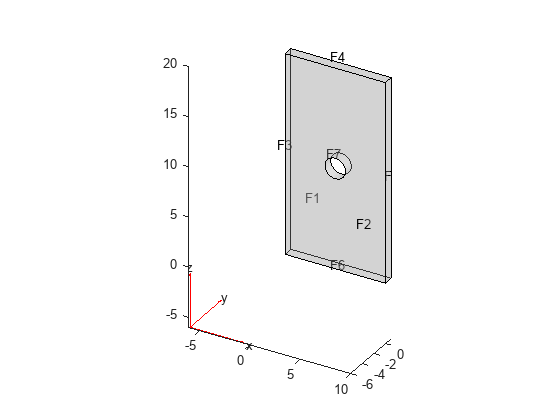
Apply the voltage boundary condition on the side faces of the geometry.

bc1 = electromagneticBC(emagmodel,"Voltage",0,"Face",3:6)

bc1 = 
  ElectromagneticBCAssignment with properties:

      RegionID: [3 4 5 6]
    RegionType: 'Face'
    Vectorized: 'off'
       Voltage: 0

Apply the voltage boundary condition on the face bordering the hole.

bc2 = electromagneticBC(emagmodel,"Voltage",1000,"Face",7)

bc2 = 
  ElectromagneticBCAssignment with properties:

      RegionID: 7
    RegionType: 'Face'
    Vectorized: 'off'
       Voltage: 1000

Specify Magnetic Potential on Boundary

Apply a magnetic potential boundary condition on the boundary of a circle.

emagmodel = createpde("electromagnetic","magnetostatic");
geometryFromEdges(emagmodel,@circleg);
electromagneticBC(emagmodel,"Edge",1,"MagneticPotential",0)

ans = 
  ElectromagneticBCAssignment with properties:

             RegionID: 1
           RegionType: 'Edge'
           Vectorized: 'off'
    MagneticPotential: 0

Specify Surface Current Density on Boundaries

Create an electromagnetic model for DC conduction analysis.

emagmodel = createpde("electromagnetic","conduction");

Import and plot a geometry representing a plate with a hole.

gm = importGeometry(emagmodel,"PlateHoleSolid.stl");
pdegplot(gm,"FaceLabels","on","FaceAlpha",0.3)

Apply the surface current density boundary condition on the front and back faces of the geometry.

electromagneticBC(emagmodel,"SurfaceCurrentDensity",100,"Face",[1 2])

ans = 
  ElectromagneticBCAssignment with properties:

                 RegionID: [1 2]
               RegionType: 'Face'
               Vectorized: 'off'
                  Voltage: []
    SurfaceCurrentDensity: 100

Specify Nonconstant Voltage on Boundary

Use a function handle to specify a boundary condition that depends on the coordinates.

Create an electromagnetic model for electrostatic analysis.

emagmodel = createpde("electromagnetic","electrostatic");

Create a unit circle geometry and include it in the model.

geometryFromEdges(emagmodel,@circleg);

Specify the voltage on the boundary using the function$\mathit{V}\left(\mathit{x},\mathit{y}\right)={\mathit{x}}^2$.

bc = @(location,~)location.x.^2;
electromagneticBC(emagmodel,"Edge",1:emagmodel.Geometry.NumEdges, ...
                            "Voltage",bc)

ans = 
  ElectromagneticBCAssignment with properties:

      RegionID: [1 2 3 4]
    RegionType: 'Edge'
    Vectorized: 'off'
       Voltage: @(location,~)location.x.^2

Specify Boundary Conditions for Harmonic Analysis

Specify an absorbing boundary condition and an electric field on a boundary for harmonic analysis.

Create an electromagnetic model for harmonic analysis.

emagmodel = createpde("electromagnetic","harmonic");

Import and plot a 2-D geometry representing a plate with a hole.

gm = importGeometry(emagmodel,"PlateHolePlanar.stl");
pdegplot(gm,"EdgeLabels","on")

Specify the electric field on the circular edge.

electromagneticBC(emagmodel,"Edge",5,"ElectricField",[10 0])

ans = 
  ElectromagneticBCAssignment with properties:

         RegionID: 5
       RegionType: 'Edge'
       Vectorized: 'off'
    ElectricField: [10 0]
    MagneticField: []

   Far Field
         FarField: []
        Thickness: []
          Scaling: 5
         Exponent: 4

Specify absorbing regions with the thickness 2 on the edges of the rectangle. Use the default attenuation rate for the absorbing regions.

electromagneticBC(emagmodel,"Edge",1:4, ...
                            "FarField","absorbing", ...
                            "Thickness",2)

ans = 
  ElectromagneticBCAssignment with properties:

         RegionID: [1 2 3 4]
       RegionType: 'Edge'
       Vectorized: 'off'
    ElectricField: [2x1 double]
    MagneticField: [2x1 double]

   Far Field
         FarField: "absorbing"
        Thickness: 2
          Scaling: 5
         Exponent: 4

Now specify the attenuation rate for the absorbing regions by using the Exponent and Scaling arguments.

electromagneticBC(emagmodel,"Edge",1:4, ...
                            "FarField","absorbing", ...
                            "Thickness",2, ...
                            "Exponent",3, ...
                            "Scaling",100)

ans = 
  ElectromagneticBCAssignment with properties:

         RegionID: [1 2 3 4]
       RegionType: 'Edge'
       Vectorized: 'off'
    ElectricField: [2x1 double]
    MagneticField: [2x1 double]

   Far Field
         FarField: "absorbing"
        Thickness: 2
          Scaling: 100
         Exponent: 3

Specify Magnetic Field on Boundary

Apply a magnetic field on the boundary of a square for harmonic analysis.

Create an electromagnetic model for harmonic analysis.

emagmodel = createpde("electromagnetic","harmonic")

emagmodel = 
  ElectromagneticModel with properties:

          AnalysisType: "harmonic"
              Geometry: []
    MaterialProperties: []
               Sources: []
    BoundaryConditions: []
    VacuumPermittivity: []
    VacuumPermeability: []
                  Mesh: []
             FieldType: "electric"

Change the field type from the default electric to magnetic.

emagmodel.FieldType = "magnetic"

emagmodel = 
  ElectromagneticModel with properties:

          AnalysisType: "harmonic"
              Geometry: []
    MaterialProperties: []
               Sources: []
    BoundaryConditions: []
    VacuumPermittivity: []
    VacuumPermeability: []
                  Mesh: []
             FieldType: "magnetic"

Include a square geometry in the model. Plot the geometry with the edge labels.

geometryFromEdges(emagmodel,@squareg);
pdegplot(emagmodel,"EdgeLabels","on")
xlim([-1.2 1.2])
ylim([-1.2 1.2])

Specify a magnetic field on the edges of the square.

electromagneticBC(emagmodel,"Edge",1:4,"MagneticField",[10 10])

ans = 
  ElectromagneticBCAssignment with properties:

         RegionID: [1 2 3 4]
       RegionType: 'Edge'
       Vectorized: 'off'
    ElectricField: []
    MagneticField: [10 10]

   Far Field
         FarField: []
        Thickness: []
          Scaling: 5
         Exponent: 4

Input Arguments

emagmodel — Electromagnetic model

ElectromagneticModel object

Electromagnetic model, specified as an ElectromagneticModel object. The model contains a geometry, a mesh, electromagnetic properties of the material, the electromagnetic sources, and the boundary conditions.

RegionType — Geometric region type

"Edge" for a 2-D model | "Face" for a 3-D model

Geometric region type, specified as "Edge" for a 2-D model or "Face" for a 3-D model.

Example: electromagneticBC(emagmodel,"Edge",1,"Voltage",100)

Data Types: char | string

RegionID — Region ID

vector of positive integers

Region ID, specified as a vector of positive integers. Find the edge or face IDs by using pdegplot with the EdgeLabels or FaceLabels name-value argument set to "on".

Data Types: double

V — Voltage

real number | function handle

Voltage, specified as a real number or a function handle. Use a function handle to specify a voltage that depends on the coordinates. For details, see More About.

The solver uses a voltage boundary condition for an electrostatic analysis.

Data Types: double | function_handle

A — Magnetic potential

real number | column vector | function handle

Magnetic potential, specified as a real number, a column vector of three elements for a 3-D model, or a function handle. Use a function handle to specify a magnetic potential that depends on the coordinates. For details, see More About.

The solver uses a magnetic potential boundary condition for a magnetostatic analysis.

Data Types: double | function_handle

E — Electric field

column vector | function handle

Electric field, specified as a column vector of two elements for a 2-D model, a vector of three elements for a 3-D model, or a function handle. Use a function handle to specify an electric field that depends on the coordinates. For details, see More About.

The solver uses an electric field boundary condition for a harmonic analysis with the electric field type.

Data Types: double | function_handle

K — Surface current density

real number | function handle

Surface current density in the direction normal to the boundary, specified as a real number or a function handle. The solver uses a surface current density boundary condition for a DC conduction analysis. Use a function handle to specify a surface current density that depends on the coordinates. For details, see More About.

Data Types: double

H — Magnetic field

column vector | function handle

Magnetic field, specified as a column vector of two elements for a 2-D model, a column vector of three elements for a 3-D model, or a function handle. Use a function handle to specify a magnetic field that depends on the coordinates. For details, see More About.

The solver uses a magnetic field boundary condition for a harmonic analysis with the magnetic field type.

Data Types: double | function_handle

h — Width of far field absorbing region

nonnegative number

Width of the far field absorbing region, specified as a nonnegative number. The solver uses an absorbing boundary condition for a harmonic analysis.

Data Types: double

e — Exponent defining attenuation rate

4 (default) | nonnegative number

Exponent defining the attenuation rate of the waves entering the absorbing region, specified as a nonnegative number. The solver uses an absorbing boundary condition for a harmonic analysis.

Data Types: double

s — Scaling parameter defining attenuation rate

5 (default) | nonnegative number

Scaling parameter defining the attenuation rate of the waves entering the absorbing region, specified as a nonnegative number. The solver uses an absorbing boundary condition for a harmonic analysis.

Data Types: double

Output Arguments

emagBC — Handle to electromagnetic boundary condition

ElectromagneticBCAssignment object

Handle to the electromagnetic boundary condition, returned as an ElectromagneticBCAssignment object. For more information, see ElectromagneticBCAssignment Properties.

More About

Specifying Nonconstant Parameters of Electromagnetic Model

In Partial Differential Equation Toolbox™, use a function handle to specify these electromagnetic parameters when they depend on the coordinates and, for a harmonic analysis, on the frequency:

• Relative permittivity of the material

• Relative permeability of the material

• Conductivity of the material

• Charge density as source (can depend on space only)

• Current density as source (can depend on space only)

• Magnetization (can depend on space only)

• Voltage on the boundary (can depend on space only)

• Magnetic potential on the boundary (can depend on space only)

• Electric field on the boundary (can depend on space only)

• Magnetic field on the boundary (can depend on space only)

• Surface current density on the boundary (can depend on space only)

For example, use function handles to specify the relative permittivity, charge density, and voltage on the boundary for emagmodel.

electromagneticProperties(emagmodel, ...
                          "RelativePermittivity", ...
                          @myfunPermittivity)
electromagneticSource(emagmodel, ...
                      "ChargeDensity",@myfunCharge, ...
                      "Face",2)
electromagneticBC(emagmodel, ...
                  "Voltage",@myfunBC, ...
                  "Edge",2)

The function must be of the form:

function emagVal = myfun(location,state)

The solver computes and populates the data in the location and state structure arrays and passes this data to your function. You can define your function so that its output depends on this data. You can use any names in place of location and state.

If you call electromagneticBC with Vectorized set to "on", then location can contain several evaluation points. If you do not set Vectorized or set Vectorized to "off", then the solver passes just one evaluation point in each call.

• location — A structure array containing these fields:

  • location.x — The x-coordinate of the point or points

  • location.y — The y-coordinate of the point or points

  • location.z — For a 3-D or an axisymmetric geometry, the z-coordinate of the point or points

  • location.r — For an axisymmetric geometry, the r-coordinate of the point or points

  Furthermore, for boundary conditions, the solver passes this data in the location structure:

  • location.nx — The x-component of the normal vector at the evaluation point or points

  • location.ny — The y-component of the normal vector at the evaluation point or points

  • location.nz — For a 3-D or an axisymmetric geometry, the z-component of the normal vector at the evaluation point or points

  • location.nr — For an axisymmetric geometry, the r-component of the normal vector at the evaluation point or points

• state — A structure array containing this field for a harmonic electromagnetic problem:

  • state.frequency - Frequency at evaluation points

Relative permittivity, relative permeability, and conductivity get this data from the solver:

• location.x, location.y, location.z, location.r

• state.frequency for a harmonic analysis

• Subdomain ID

Charge density, current density, magnetization, surface current density on the boundary, and electric or magnetic field on the boundary get this data from the solver:

• location.x, location.y, location.z, location.r

• Subdomain ID

Voltage or magnetic potential on the boundary get these data from the solver:

• location.x, location.y, location.z, location.r

• location.nx, location.ny, location.nz, location.nr

When you solve an electrostatic, magnetostatic, or DC conduction problem, the output returned by the function handle must be of the following size. Here, Np = numel(location.x) is the number of points.

• 1-by-Np if a function specifies the nonconstant relative permittivity, relative permeability, or charge density. For the charge density, the output can also be Np-by-1.

• 1-by-Np for a 2-D model and 3-by-Np for a 3-D model if a function specifies the nonconstant current density and magnetic potential on the boundary. For the current density, the output can also be Np-by-1 or Np-by-3.

• 2-by-Np for a 2-D model and 3-by-Np for a 3-D model if a function specifies the nonconstant magnetization or surface current density on the boundary.

When you solve a harmonic problem, the output returned by the function handle must be of the following size. Here, Np = numel(location.x) is the number of points.

• 1-by-Np if a function specifies the nonconstant relative permittivity, relative permeability, and conductivity.

• 2-by-Np for a 2-D problem and 3-by-Np for a 3-D problem if a function specifies the nonconstant electric or magnetic field.

• 2-by-Np or Np-by-2 for a 2-D problem and 3-by-Np or Np-by-3 for a 3-D problem if a function specifies the nonconstant current density and the field type is electric.

• 1-by-Np or Np-by-1 for a 2-D problem and 3-by-Np or Np-by-3 for a 3-D problem if a function specifies the nonconstant current density and the field type is magnetic.

If relative permittivity, relative permeability, or conductivity for a harmonic analysis depends on the frequency, ensure that your function returns a matrix of NaN values of the correct size when state.frequency is NaN. Solvers check whether a problem is nonlinear by passing NaN state values and looking for returned NaN values.

Additional Arguments in Functions for Nonconstant Electromagnetic Parameters

To use additional arguments in your function, wrap your function (that takes additional arguments) with an anonymous function that takes only the location and state arguments. For example:

emagVal = @(location,state) myfunWithAdditionalArgs(location,arg1,arg2,...)
electromagneticBC(model,"Edge",3,"Voltage",emagVal)

Version History

Introduced in R2021a

R2022b: Surface current density

Surface current density boundary condition can be specified for a DC conduction analysis.

R2022a: Boundary conditions for harmonic analysis

Electric and magnetic field on boundaries, and absorbing boundary conditions can be specified for harmonic analysis.

R2021b: Support for 3-D electrostatic and magnetostatic problems

Voltage and magnetic potential can be specified on faces for 3-D electrostatic and magnetostatic problems.