Plot Functions

Plot Optimization During Execution

You can plot various measures of progress during the execution of a solver. Use the PlotFcn name-value argument of optimoptions to specify one or more plotting functions for the solver to call at each iteration. Pass a function handle, function name, or cell array of function handles or function names as the PlotFcn value.

Each solver has a variety of predefined plot functions available. For more information, see the PlotFcn option description on the function reference page for a solver.

You can also use a custom plot function, as shown in Create Custom Plot Function. Write a function file using the same structure as an output function. For more information on this structure, see Output Function and Plot Function Syntax.

Use Predefined Plot Functions

This example shows how to use plot functions to view the progress of the fmincon "interior-point" algorithm. The problem is taken from Constrained Nonlinear Problem Using Optimize Live Editor Task or Solver.

Write the nonlinear objective and constraint functions, including their gradients. The objective function is Rosenbrock's function.

type rosenbrockwithgrad

function [f,g] = rosenbrockwithgrad(x)
% Calculate objective f
f = 100*(x(2) - x(1)^2)^2 + (1-x(1))^2;

if nargout > 1 % gradient required
    g = [-400*(x(2)-x(1)^2)*x(1)-2*(1-x(1));
        200*(x(2)-x(1)^2)];
end

Save this file as rosenbrockwithgrad.m.

The constraint function is that the solution satisfies norm(x)^2 <= 1.

type unitdisk2

function [c,ceq,gc,gceq] = unitdisk2(x)
c = x(1)^2 + x(2)^2 - 1;
ceq = [ ];

if nargout > 2
    gc = [2*x(1);2*x(2)];
    gceq = [];
end

Save this file as unitdisk2.m.

Create options for the solver that include calling three plot functions.

options = optimoptions(@fmincon,Algorithm="interior-point",...
 SpecifyObjectiveGradient=true,SpecifyConstraintGradient=true,...
 PlotFcn={@optimplotx,@optimplotfval,@optimplotfirstorderopt});

Create the initial point x0 = [0,0], and set the remaining inputs to empty ([]).

x0 = [0,0];
A = [];
b = [];
Aeq = [];
beq = [];
lb = [];
ub = [];

Call fmincon, including the options.

fun = @rosenbrockwithgrad;
nonlcon = @unitdisk2;
x = fmincon(fun,x0,A,b,Aeq,beq,lb,ub,nonlcon,options)

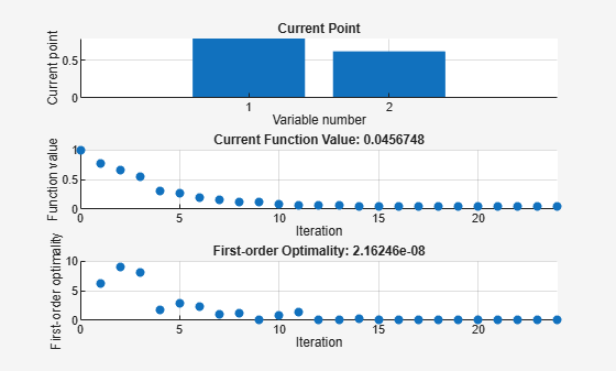
Local minimum found that satisfies the constraints.

Optimization completed because the objective function is non-decreasing in 
feasible directions, to within the value of the optimality tolerance,
and constraints are satisfied to within the value of the constraint tolerance.

x = 1×2

    0.7864    0.6177

Create Custom Plot Function

To create a custom plot function for an Optimization Toolbox™ solver, write a function using the syntax

function stop = plotfun(x,optimValues,state)
stop = false;
switch state
    case "init"
        % Set up plot
    case "iter"
        % Plot points
    case "done"
        % Clean up plots
    % Some solvers also use case "interrupt"
end
end

Global Optimization Toolbox solvers use different syntaxes.

The software passes the x, optimValues, and state data to your plot function. For complete syntax details and a list of the data in the optimValues argument, see Output Function and Plot Function Syntax. You pass the plot function name to the solver using the PlotFcn name-value argument.

For example, the plotfandgrad helper function listed at the end of this example plots the objective function value and norm of the gradient for a scalar-valued objective function. Use the ras helper function listed at the end of this example as the objective function. The ras function includes a gradient calculation, so for efficiency, set the SpecifyObjectiveGradient name-value argument to true.

fun = @ras;
rng(1) % For reproducibility
x0 = 10*randn(2,1); % Random initial point
opts = optimoptions(@fminunc,SpecifyObjectiveGradient=true,PlotFcn=@plotfandgrad);
[x,fval] = fminunc(fun,x0,opts)

Local minimum found.

Optimization completed because the size of the gradient is less than
the value of the optimality tolerance.

x = 2×1

    1.9949
    1.9949

fval = 
17.9798

The plot shows that the norm of the gradient converges to zero, as expected for an unconstrained optimization.

Helper Functions

This code creates the plotfandgrad helper function.

function stop = plotfandgrad(x,optimValues,state)
persistent iters fvals grads % Retain these values throughout the optimization
stop = false;

switch state
    case "init"
        iters = [];
        fvals = [];
        grads = [];
    case "iter"
        iters = [iters optimValues.iteration];
        fvals = [fvals optimValues.fval];
        grads = [grads norm(optimValues.gradient)];
        plot(iters,fvals,"o",iters,grads,"x");
        legend("Objective","Norm(gradient)")
    case "done"
end
end

This code creates the ras helper function.

function [f,g] = ras(x)
f = 20 + x(1)^2 + x(2)^2 - 10*cos(2*pi*x(1) + 2*pi*x(2));
if nargout > 1
    g(2) = 2*x(2) + 20*pi*sin(2*pi*x(1) + 2*pi*x(2));
    g(1) = 2*x(1) + 20*pi*sin(2*pi*x(1) + 2*pi*x(2));
end
end

Related Topics

• Output Function and Plot Function Syntax
• Output Function for Problem-Based Optimization
• intlinprog Output Function and Plot Function Syntax