Design Controller Using MPC Designer

This example shows how to design a model predictive controller for a continuous stirred-tank reactor (CSTR) using MPC Designer.

CSTR Model

The linearized model of a Continuously Stirred Tank Reactor (CSTR) is shown in CSTR Model. In the model, the first two state variables are the concentration of reagent (here referred to as C_A and measured in kmol/m³) and the temperature of the reactor (here referred to as T, measured in K), while the first two inputs are the coolant temperature (T_c, measured in K, used to control the plant), and the inflow feed reagent concentration C_Af measured in kmol/m³, (often considered as unmeasured disturbance).

For this example, the coolant temperature has a limited range of ±10 degrees from its nominal value and a limited rate of change of ±2 degrees per second.

Create a state-space model of a CSTR system.

A = [   -5  -0.3427;
     47.68    2.785];
B = [    0   1
       0.3   0];
C = flipud(eye(2));
D = zeros(2);
CSTR = ss(A,B,C,D);

Import Plant and Define MPC Structure

mpcDesigner

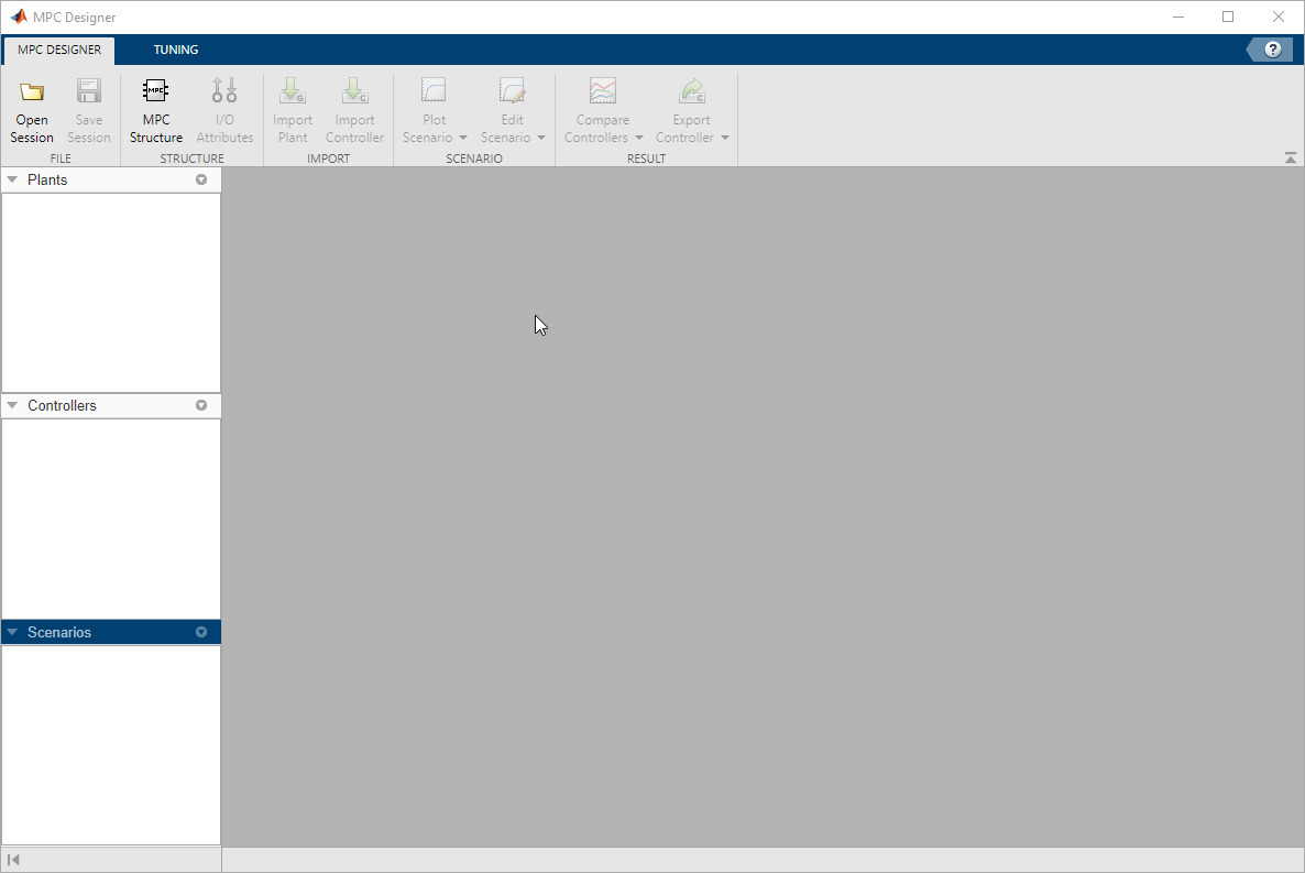
On the MPC Designer tab, in the Structure section, click MPC Structure.

In the Define MPC Structure By Importing dialog box, in the Select a plant model or an MPC controller from MATLAB workspace table, select the CSTR model.

Since CSTR is a stable, continuous-time LTI system, MPC Designer sets the controller sample time to 0.1 T_r, where T_r is the average rise time of CSTR. For this example, in the Specify MPC controller sample time field, enter a sample time of 0.5 seconds.

By default, all plant inputs are defined as manipulated variables and all plant outputs as measured outputs. In the Assign plant i/o channels section, assign the input and output channel indices such that:

• The first input, coolant temperature, is a manipulated variable.

• The second input, feed concentration, is an unmeasured disturbance.

• The first output, reactor temperature, is a measured output.

• The second output, reactant concentration, is an unmeasured output.

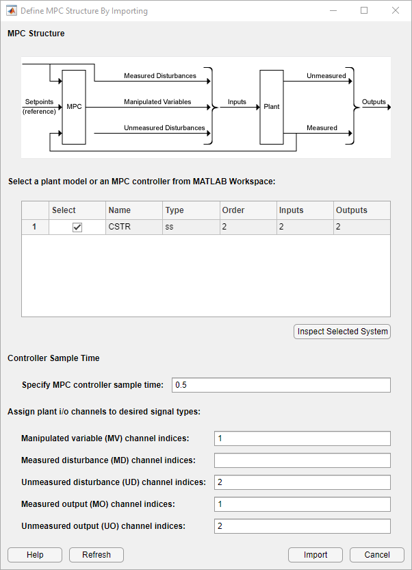
Click Import.

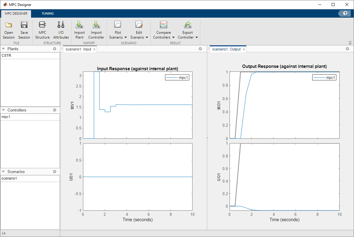
The app imports the CSTR plant to the Data Browser. The following are also added to the Data Browser:

• mpc1 — Default MPC controller created using CSTR as its internal model.

• scenario1 — Default simulation scenario.

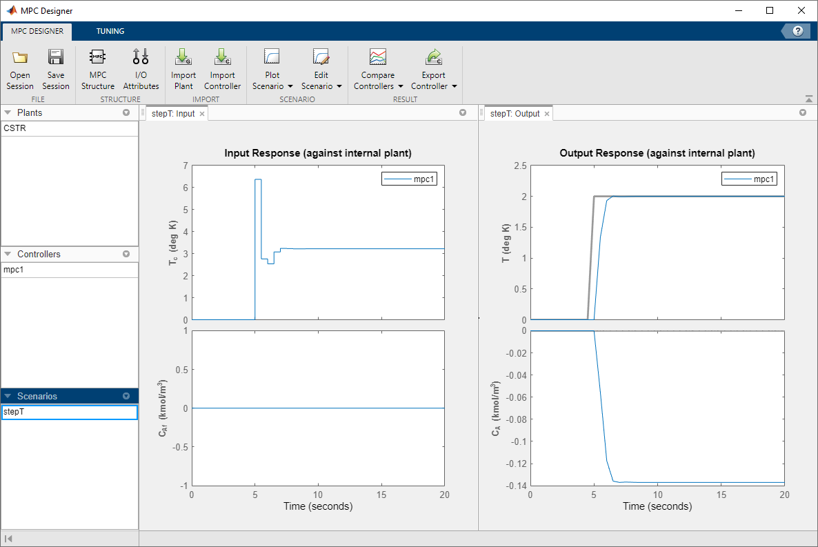
The app runs the default simulation scenario and updates the Input Response and Output Response plots. The closed loop system is able to track the desired measured output successfully, while this is not the case for the unmeasured output. This behavior is expected as the plant has only one manipulated variable.

Once you define the MPC structure, you cannot change it within the current MPC Designer session. To use a different channel configuration, start a new session of the app.

Define Input and Output Channel Attributes

On the MPC Designer tab, select I/O Attributes.

In the Input and Output Channel Specifications dialog box, in the Name column, specify a meaningful name for each input and output channel.

In the Unit column, optionally specify the units for each channel.

Since the state-space model is defined using deviations from the nominal operating point, keep the Nominal Value for each input and output channel to 0.

Keep the Scale Factor for each channel at the default value of 1.

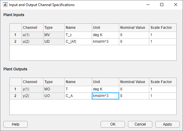
Click OK.

The Input Response and Output Response plot labels update to reflect the new signal names and units.

Configure Simulation Scenario

On the MPC Designer tab, in the Scenario section, click Edit Scenario > scenario1.

In the Simulation Scenario dialog box, set the Simulation duration to 20 seconds.

In the Reference Signals table, in the first row, specify a step Size of 2 and a Time of 5.

In the Signal column, in the second row, select a Constant reference to hold the concentration setpoint at its nominal value, defined in the Input and Output Channel Specifications dialog box (in this case the nominal value is zero).

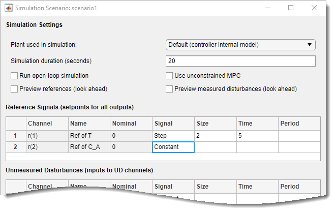
The default scenario is configured to simulate a step change of 2 degrees Kelvin in the reference reactor temperature, T, at a time of 5 seconds.

Click OK.

The response plots update to reflect the new simulation scenario configuration. The reference value for C_A is no longer a step but a constant equal to zero.

In the Scenarios section in the lower left part of MPC Designer, click scenario1. Click scenario1 a second time, and rename the scenario to stepT.

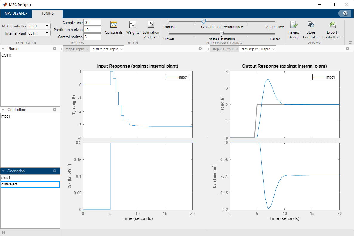
Configure Controller Horizons

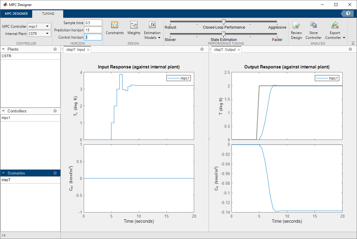
On the Tuning tab, in the Horizons section, specify a Prediction horizon of 15 and a Control horizon of 3.

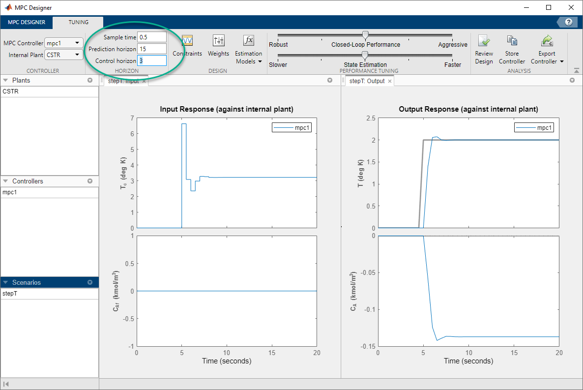
The response plots update to reflect the new horizons. The Input Response plot shows that the control actions violate the required constraint on the rate of change for the coolant temperature.

Define Input Constraints

In the Design section, click Constraints.

In the Constraints dialog box, in the Input and Output Constraints section, in the Inputs row, enter the coolant temperature upper and lower bounds in the Min and Max columns respectively.

Specify the rate of change limits in the RateMin and RateMax columns.

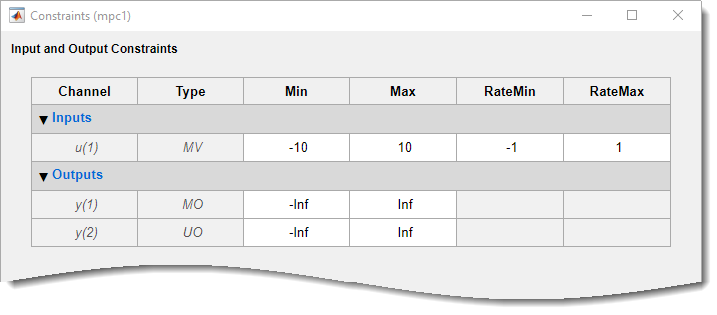
Click OK.

The Input Response plot shows the constrained manipulated variable control actions.

Specify Controller Tuning Weights

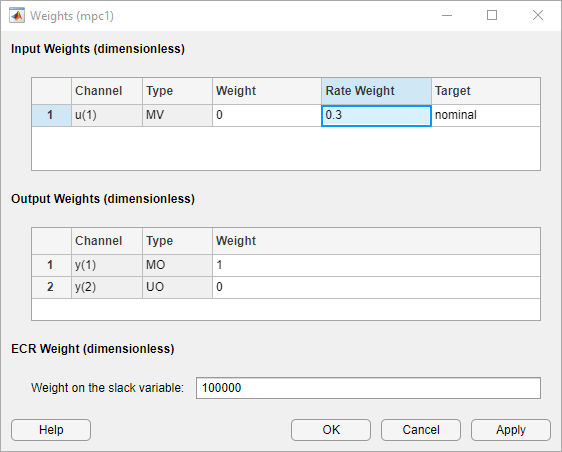
On the Tuning tab, in the Design section, click Weights.

In the Input Weights table, increase the manipulated variable (MV) Rate Weight to 0.3. Increasing the MV rate weight penalizes large MV changes in the controller optimization cost function.

In the Output Weights table, keep the default Weight values. By default, all unmeasured outputs have zero weights.

Since there is only one manipulated variable, if the controller tries to hold both outputs at specific setpoints, one or both outputs will exhibit steady-state error in their responses. Since the controller ignores setpoints for outputs with zero weight, setting the concentration output weight to zero allows reactor temperature setpoint tracking with zero steady-state error.

Click OK.

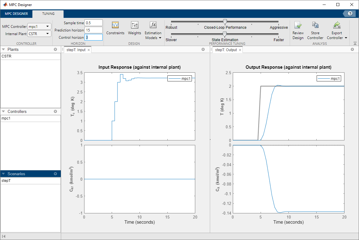
The Input Response plot shows the more conservative control actions, which result in a slower Output Response.

Eliminate Output Overshoot

Suppose the application demands zero overshoot in the output response. On the Performance Tuning tab, drag the Closed-Loop Performance slider to the left until the Output Response has no overshoot. Moving this slider to the left simultaneously increases the manipulated variable rate weight of the controller and decreases the output variable weight, producing a more robust controller.

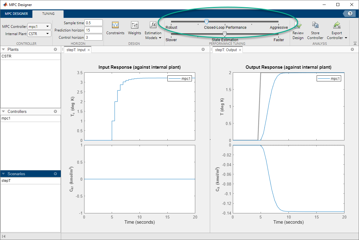
When you adjust the controller tuning weights using the Closed-Loop Performance slider, MPC Designer does not change the weights you specified in the Weights dialog box. Instead, the slider controls an adjustment factor, which is used with the user-specified weights to define the actual controller weights.

This factor is 1 when the slider is centered; its value decreases as the slider moves left and increases as the slider moves right. The weighting factor multiplies the manipulated variable and output variable weights and divides the manipulated variable rate weights from the Weights dialog box. Therefore, moving the slider to increase robustness decreases both OV and MV weights and increases MV Rate weights, which leads to relaxed control of outputs and more conservative control moves.

To view the actual controller weights, export the controller to the MATLAB^® workspace, and view the Weights property of the exported controller object.

Test Controller Disturbance Rejection

In a process control application, disturbance rejection is often more important than setpoint tracking. Simulate the controller response to a step change in the feed concentration unmeasured disturbance.

On the MPC Designer tab, in the Scenario section, click Plot Scenario > New Scenario.

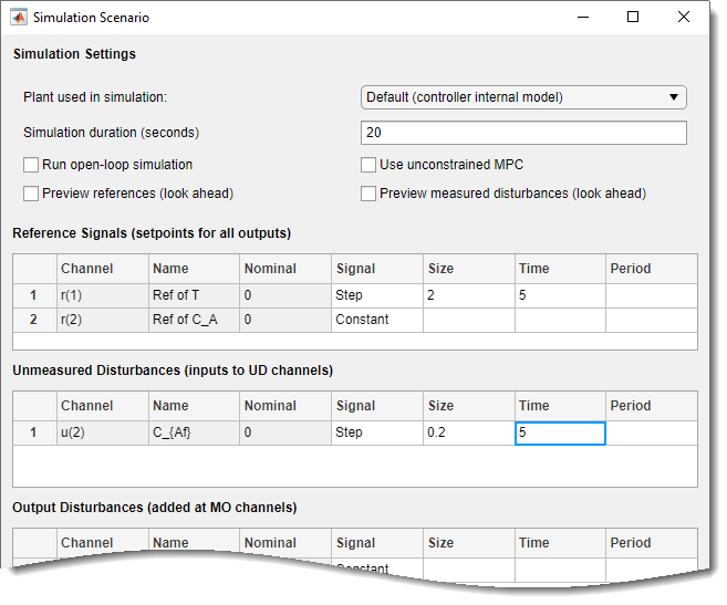
In the Simulation Scenario dialog box, set the Simulation duration to 20 seconds.

In the Reference Signals table, in the first row, in the Signal drop-down list, select Step, then specify a step Size of 2, and a Time of 5. In the Signal column, in the second row, keep a Constant reference to hold the concentration setpoint at its nominal value.

In the Unmeasured Disturbances row, in the Signal drop-down list, select Step. then specify a step Size of 0.2 and a Time of 5.

Click OK.

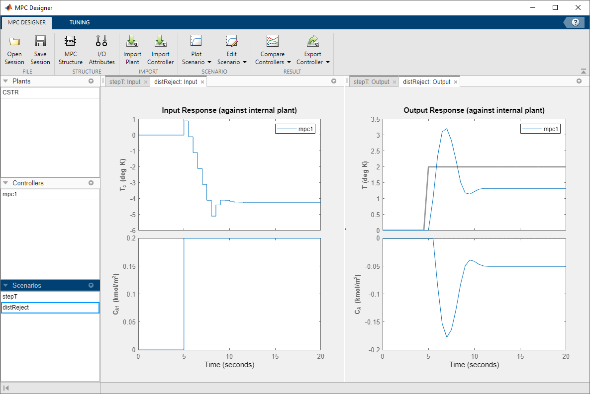
The app adds new scenario to the Data Browser and creates new corresponding Input Response and Output Response plots.

In the Data Browser, in the Scenarios section, rename NewScenario to distReject.

As you can see from the Output Response plots, the closed-loop system is still able to reach the desired reactor temperature. In this case, the required control actions, combined with the input disturbance, cause a steady-state decrease in the output concentration, C_A of 0.1 kmol/m³.

Specify Concentration Output Constraint

Previously, you defined the controller tuning weights to achieve the primary control objective of tracking the reactor temperature setpoint with zero steady-state error. Doing so enables the unmeasured reactor concentration to vary freely. Suppose that unwanted reactions occur once the reactor concentration drops below 0.05 kmol/m³ with respect to its nominal value. To constrain the reactor concentration, specify an output constraint.

On the Tuning tab, in the Design section, click Constraints.

In the Constraints dialog box, in the Input and Output Constraints sections, in second row of the Outputs table, specify a Min unmeasured output (UO) value of -0.05.

By default, all output constraints are soft, meaning that their MinECR and MaxECR values are greater than zero. To soften the unmeasured output (UO) constraint further, increase its MaxECR value.

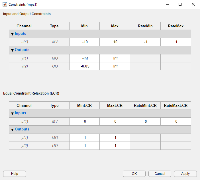
Click OK.

In the Output Response plots, the reactor concentration, C_A, stabilizes at -0.05 kmol/m³ after 10 seconds. Since there is only one manipulated variable, the controller makes a compromise between the two competing control objectives: Temperature tracking and constraint satisfaction. A softer output constraint enables the controller to sacrifice the constraint requirement more to improve the temperature tracking.

Since the output constraint is soft, the controller maintains some level of temperature control by allowing small concentration constraint violations. In general, depending on your application requirements, you can experiment with different constraint settings to achieve an acceptable control objective compromise.

Export Controller

In the Tuning tab, in the Analysis section, click Export Controller to save the tuned controller, mpc1, to the MATLAB workspace.

Delete Plants, Controllers, and Scenarios

To delete a plant, controller, or scenario, in the Data Browser, right-click the item you want to delete, and select Delete.

You cannot delete the current controller. Also, you cannot delete a plant or scenario if it is the only listed plant or scenario.

If a plant is used by any controller or scenario, you cannot delete the plant.

To delete multiple plants, controllers, or scenarios, hold Shift and click each item that you want to delete.

References

[1] Seborg, D. E., T. F. Edgar, and D. A. Mellichamp, Process Dynamics and Control, 2nd Edition, Wiley, 2004, pp. 34–36 and 94–95.