Align Brain MRI and Dynamic PET Data
This example shows how to align anatomical brain MRI and resting state dynamic PET data.
Fluorodeoxyglucose positron emission tomography (FDG-PET) involves introducing the radiotracer fluorodeoxyglucose into the body. The amount of FDG that accumulates in the tissue depends on the amount of glucose utilized by the tissue and provides information about the health of the tissue. Magnetic resonance imaging (MRI) uses a magnetic field to disturb the magnetic equilibrium of hydrogen nuclei in the body and measure the time taken by the hydrogen nuclei to regain equilibrium. While MRI has many uses in understanding the structure of tissues, the main use of PET is for the diagnosis and tracking of cancer. While dynamic PET is a 4-D spatiotemporal volume that measures the accumulation of FDG in each voxel as a function of time, static PET is a 3-D spatial volume that represents the accumulation of FDG over the entire duration of the scan.
An anatomical brain MRI is a 3-D image of the brain, and a dynamic PET is a 4-D spatiotemporal volume of the brain. In this example, you perform these steps to align dynamic PET data and an anatomical brain MRI.
Preprocess the dynamic PET data.
Compute a static PET volume from the dynamic PET data.
Resample the static PET volume to align with the anatomical brain MRI
Resample the dynamic PET data to align with the anatomical brain MRI
Download Data Set
This example uses dynamic PET and anatomical MRI images of one subject from the Monash rsPET-MR data set [1]. The data was obtained from the OpenNeuro database [2].
Download and unzip the data set.
zipFile = matlab.internal.examples.downloadSupportFile("medical","restingBrainPETMR.zip");
filepath = fileparts(zipFile);
unzip(zipFile,filepath)
Load Dynamic PET Data
Import the dynamic PET data as a medicalVolume object. Observe that the 4-D spatiotemporal volume has a spatial size of 344-by-344-by-127 and 356 timepoints.
filename = fullfile(filepath,"sub-01_task-rest_pet.nii.gz");
dynamicPET = medicalVolume(filename)
dynamicPET =
medicalVolume with properties:
Voxels: [344×344×127×356 single]
VolumeGeometry: [1×1 medicalref3d]
SpatialUnits: "mm"
Orientation: "transverse"
VoxelSpacing: [1.3908 1.3908 2.0312]
NormalVector: [0 0 -1]
NumCoronalSlices: 344
NumSagittalSlices: 344
NumTransverseSlices: 127
PlaneMapping: ["sagittal" "coronal" "transverse"]
Modality: "unknown"
WindowCenters: 0
WindowWidths: 0
spatialSizePET = dynamicPET.VolumeGeometry.VolumeSize
spatialSizePET = 1×3

    344    344    127
numTimepointsPET = size(dynamicPET.Voxels,4)
numTimepointsPET =
356
Preprocess Dynamic PET Data
Extract the voxels of the dynamic PET data.
dynamicPETVoxels = dynamicPET.Voxels;
Spatially smooth the 3-D volume at each timepoint of the 4-D spatiotemporal volume with a Gaussian kernel having a width of 7 voxels and a standard deviation of 1 voxel, as recommended for the data set [3].
s_width = 7;
s_sigma = 1;
kernel = fspecial3("gaussian",s_width,s_sigma);
for t = 1:numTimepointsPET
    dynamicPETVoxels(:,:,:,t) = convn(dynamicPETVoxels(:,:,:,t),kernel,"same");
end
The temporal resolution of the dynamic PET data is 16 seconds, making the entire PET scan duration across 356 timepoints equal to approximately 90 minutes. Retain only the last 225 timepoints, equivalent to the last 60 minutes of PET acquisition, when the infusion of the radiotracer has reached all parts of the brain.
dynamicPETVoxels = dynamicPETVoxels(:,:,:,end-225+1:end);
Create a medicalVolume object of the preprocessed dynamic PET data.
dynamicPETPreprocessed = medicalVolume(dynamicPETVoxels,dynamicPET.VolumeGeometry)
dynamicPETPreprocessed =
  medicalVolume with properties:

                 Voxels: [344×344×127×225 single]
         VolumeGeometry: [1×1 medicalref3d]
           SpatialUnits: "unknown"
            Orientation: "transverse"
           VoxelSpacing: [1.3908 1.3908 2.0312]
           NormalVector: [0 0 -1]
       NumCoronalSlices: 344
      NumSagittalSlices: 344
    NumTransverseSlices: 127
           PlaneMapping: ["sagittal"    "coronal"    "transverse"]
               Modality: "unknown"
          WindowCenters: []
           WindowWidths: []
numTimepointsPET = size(dynamicPETPreprocessed.Voxels,4)
numTimepointsPET =
225
Compute Static PET Image from Dynamic PET Data
Compute the 3-D static PET volume, from the preprocessed 4-D dynamic PET data, as the accumulation of the radiotracer over time.
staticPETVoxels = sum(dynamicPETPreprocessed.Voxels,4);
Create a medicalVolume object of the static PET volume for ease of visualization.
staticPET = medicalVolume(staticPETVoxels,dynamicPET.VolumeGeometry)
staticPET =
  medicalVolume with properties:

                 Voxels: [344×344×127 single]
         VolumeGeometry: [1×1 medicalref3d]
           SpatialUnits: "unknown"
            Orientation: "transverse"
           VoxelSpacing: [1.3908 1.3908 2.0312]
           NormalVector: [0 0 -1]
       NumCoronalSlices: 344
      NumSagittalSlices: 344
    NumTransverseSlices: 127
           PlaneMapping: ["sagittal"    "coronal"    "transverse"]
               Modality: "unknown"
          WindowCenters: []
           WindowWidths: []
Visualize the static PET volume.
figure
sliceViewer(staticPET,Colormap=jet(256))

Load Anatomical MRI
Import the anatomical MRI as a medicalVolume object. Observe that the 3-D volume has a spatial size of 176-by-256-by-256, which is different than that of the PET data.
filename = fullfile(filepath,"sub-01_T1w.nii.gz");
anatMRI = medicalVolume(filename);
spatialSizeMRI = anatMRI.VolumeGeometry.VolumeSize
spatialSizeMRI = 1×3
176 256 256
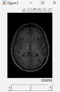
Visualize the anatomical MRI volume.
figure
sliceViewer(anatMRI)
Align Static and Dynamic PET to Anatomical MRI
Because the PET and MRI data have been acquired simultaneously using a single scanner [1], resampling is enough to align the PET and MRI data. Resample the static PET volume to match the anatomical MRI volume geometry.
staticPETResampled = resample(staticPET,anatMRI.VolumeGeometry)
staticPETResampled =
  medicalVolume with properties:

                 Voxels: [176×256×256 single]
         VolumeGeometry: [1×1 medicalref3d]
           SpatialUnits: "unknown"
            Orientation: "transverse"
           VoxelSpacing: [1.0000 1.0000 1.0000]
           NormalVector: [0.0313 1.6248e-04 0.9995]
       NumCoronalSlices: 256
      NumSagittalSlices: 176
    NumTransverseSlices: 256
           PlaneMapping: ["sagittal"    "coronal"    "transverse"]
               Modality: "unknown"
          WindowCenters: []
           WindowWidths: []
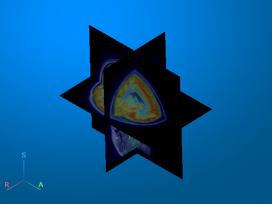
Visualize the resampled static PET volume overlaid on the anatomical MRI volume. Observe that resampling has aligned the static PET and anatomical MRI volumes.
viewer = viewer3d;
overlayData = staticPETResampled.Voxels;
overlayRange = max(anatMRI.Voxels,[],"all");
overlayData = overlayData/single(overlayRange);
volshow(anatMRI,Parent=viewer,RenderingStyle="SlicePlanes",Colormap=gray, ...
    OverlayData=overlayData,OverlayRenderingStyle="VolumeOverlay",OverlayColormap=jet)

Similarly align the dynamic PET data, by resampling each timepoint of the spatiotemporal volume.
dynamicPETResampledVoxels = [];
for t = 1: numTimepointsPET
    singleTimepointPET = medicalVolume(dynamicPETPreprocessed.Voxels(:,:,:,t), ...
        dynamicPETPreprocessed.VolumeGeometry);
    singleTimepointPET = resample(singleTimepointPET,anatMRI.VolumeGeometry);
    dynamicPETResampledVoxels = cat(4,dynamicPETResampledVoxels,singleTimepointPET.Voxels);
end
dynamicPETResampled = medicalVolume(dynamicPETResampledVoxels,staticPETResampled.VolumeGeometry)
dynamicPETResampled =
  medicalVolume with properties:

                 Voxels: [176×256×256×225 single]
         VolumeGeometry: [1×1 medicalref3d]
           SpatialUnits: "unknown"
            Orientation: "transverse"
           VoxelSpacing: [1.0000 1.0000 1.0000]
           NormalVector: [0.0313 1.6248e-04 0.9995]
       NumCoronalSlices: 256
      NumSagittalSlices: 176
    NumTransverseSlices: 256
           PlaneMapping: ["sagittal"    "coronal"    "transverse"]
               Modality: "unknown"
          WindowCenters: []
           WindowWidths: []
References
[1] Jamadar, Sharna D., Phillip G. D. Ward, Thomas G. Close, Alex Fornito, Malin Premaratne, Kieran O’Brien, Daniel Stäb, Zhaolin Chen, N. Jon Shah, and Gary F. Egan. “Simultaneous BOLD-fMRI and Constant Infusion FDG-PET Data of the Resting Human Brain.” Scientific Data 7, no. 1 (October 21, 2020): 363. https://doi.org/10.1038/s41597-020-00699-5.
[2] Jamadar, Sharna D., Phillip G.D. Ward, Thomas G. Close, Alex Fornito, Malin Premaratne, Kieren O’Brien, Daniel Staeb, Zhaolin Chen, N. Jon Shah, and Gary F. Egan. “Monash rsPET-MR”. Openneuro, 2023. https://doi.org/10.18112/OPENNEURO.DS002898.V1.4.0.
[3] Jamadar, Sharna D., Phillip G. D. Ward, Emma X. Liang, Edwina R. Orchard, Zhaolin Chen, and Gary F. Egan. “Metabolic and Hemodynamic Resting-State Connectivity of the Human Brain: A High-Temporal Resolution Simultaneous BOLD-fMRI and FDG-fPET Multimodality Study.” Cerebral Cortex (New York, N.Y.: 1991) 31, no. 6 (May 10, 2021): 2855–67. https://doi.org/10.1093/cercor/bhaa393.