Gasoline Case Study

This example uses:

This example shows how to automatically generate an mbcmodel project for the gasoline case study using the command-line functions. First, you create and load data into a project. Next, you build a test plan, boundary models, and responses. Then you remove data outliers and create feature models. Finally, you make a two-stage model and plot torque versus spark. The example uses the DIVCP_Main_DoE_Data.mat file in the mbctraining folder.

Create a New `mbcmodel` Project

Use the CreateProject function to create a project.

project = mbcmodel.CreateProject;

Load Data into Project

Use functions to group data into tests, remove bad data, and remove tests that do not have enough data to fit local models.

datafile = fullfile( mbcpath, 'mbctraining', 'DIVCP_Main_DoE_Data.mat' );
data = CreateData( project, datafile );

BeginEdit( data );

% Group data by test number GDOECT.
DefineTestGroups( data, 'GDOECT', 0.5, 'GDOECT', false );
% Get rid of data which is probably unstable.
AddFilter( data, 'RESIDFRAC < 35' );
AddFilter( data, 'AFR > 14.25' );
% Get rid of the tests that are too small.
AddTestFilter( data, 'length(BTQ) > 4' );

% Commit the changes to the project.
CommitEdit( data );

Build Test Plan

Define the inputs for the test plan.

LocalInputs = mbcmodel.modelinput('Symbol','S',...
    'Name','SPARK',...
    'Range',[0 50]);
GlobalInputs = mbcmodel.modelinput('Symbol',{'N','L','ICP','ECP'},...
    'Name',{'SPEED','LOAD','INT_ADV','EXH_RET'},...
    'Range',{[500 6000],[0.0679    0.9502],[-5 50],[-5 50]});
% Create test plan.
testplan = CreateTestplan( project, {LocalInputs,GlobalInputs} );
% Attach data to the test plan.
AttachData( testplan, data );

Build Boundary Models

Create a global boundary model and add it to the test plan tree.

B = CreateBoundary(testplan.Boundary.Global,'Star-shaped');
% Add boundary model to the test plan. The boundary model is fitted when it
% is added to the boundary model tree. The boundary model is included in
% the best boundary model for the tree by default. 
% All inputs are used in the boundary model by default.
B = Add(testplan.Boundary.Global,B);

% Make a boundary model using only speed and load and add to the
% boundary tree. 
B.ActiveInputs = [true true false false];
B = Add(testplan.Boundary.Global,B);
% Look at the global boundary tree.
testplan.Boundary.Global

ans = 
  Tree with properties:

         Data: [189×4 double]
       Models: {[1×1 mbcboundary.Model]  [1×1 mbcboundary.Model]}
    BestModel: [1×1 mbcboundary.Boolean]
       InBest: [1 1]
     TestPlan: [1×1 mbcmodel.testplan]

Build Responses

Build response models for torque, exhaust temperature and residual fraction. Use a local polynomial spline model for torque. For the exhaust temperature and residual fraction, use a local polynomial model with datum.

LocalTorque  = mbcmodel.CreateModel('Local Polynomial Spline',1);
LocalTorque.Properties.LowOrder = 2;
% Use the default global model.
GlobalModel = testplan.DefaultModels{2};
CreateResponse(testplan,'BTQ',LocalTorque,GlobalModel,'Maximum');
% make exhaust temperature and residual fraction models
LocalPoly  = mbcmodel.CreateModel('Local Polynomial with Datum',1);
CreateResponse(testplan,'EXTEMP',LocalPoly,GlobalModel,'Linked');
CreateResponse(testplan,'RESIDFRAC',LocalPoly,GlobalModel,'Linked');

Remove Local Outliers

Remove data if abs(studentized residuals) > 3. The Gasoline_project uses a different process to decide which outliers to remove.

TQ_response = testplan.Responses(1);
numTests = TQ_response.NumberOfTests;
LocalBTQ = TQ_response.LocalResponses;
for tn = 1:numTests
    % Find observations with studentized residuals greater than 3
    studentRes = DiagnosticStatistics( LocalBTQ, tn, 'Studentized residuals' );
    potentialOut  = abs( studentRes )> 3;
    if any(potentialOut)
        % Don't update response feature models until end of loop
        RemoveOutliersForTest( LocalBTQ, tn, potentialOut , false);
    end
    % get local model for test and look at summary statistics
    mdl = ModelForTest(LocalBTQ,tn);
    if ~strcmp(mdl.Status,'Not fitted')
        LocalStats = SummaryStatistics(mdl);
    end
end

Update the response features.

UpdateResponseFeatures(LocalBTQ);

Remove Points Where MBT<0 or MBT>60

Remove points where the maximum brake torque (MBT) is less than 0 or greater than 60.

knot = LocalBTQ.ResponseFeatures(1);
PointsToRemove = knot.DoubleResponseData<0 | knot.DoubleResponseData>60;
knot.RemoveOutliers(PointsToRemove);

Create Alternative Response Feature Models

Make a list of these alternative response feature models. Select the best model, based on the Akaike Information Criteria (AICc).

Quadratic
Cubic
RBF with a range of centers
Polynomial-RBF with a range of centers

Get the base model. You use this to create the other models.

rf = LocalBTQ.ResponseFeatures(1);
BaseModel = rf(1).Model;

Make a quadratic model that uses Minimize PRESS to fit. Add it to the list.

m = BaseModel.CreateModel('Polynomial');
m.Properties.Order = [2 2 2 2];
m.FitAlgorithm = 'Minimize PRESS';
mlist = {m};

Make a cubic model and add it to the list.

m.Properties.Order = [3 3 3 3];
m.Properties.InteractionOrder = 2;
mlist{2} = m;

Make RBF models with a range of centers. The maximum number of centers is set in the center selection algorithm.

m = BaseModel.CreateModel('RBF');
Centers = [50 80];
Start = length(mlist);
mlist = [mlist cell(size(Centers))];
for i = 1:length(Centers)
    fitAlgorithm = m.FitAlgorithm.WidthAlgorithm.NestedFitAlgorithm;
    fitAlgorithm.CenterSelectionAlg.MaxCenters = Centers(i);
    m.FitAlgorithm.WidthAlgorithm.NestedFitAlgorithm = fitAlgorithm;
    mlist{Start+i} = m;
end

Make Polynomial-RBF models with a range of centers.

m = BaseModel.CreateModel('Polynomial-RBF');
m.Properties.Order = [2 2 2 2];
Start = length(mlist);
mlist = [mlist cell(size(Centers))];
for i = 1:length(Centers)
    % Maximum number of centers is set in the nested fit algorithm
    m.FitAlgorithm.WidthAlgorithm.NestedFitAlgorithm.MaxCenters = Centers(i);
    mlist{Start+i} = m;
end

Make alternative models for each response feature and select the best model, based on AICc.

criteria = 'AICc';
CreateAlternativeModels( LocalBTQ, mlist, criteria );

Alter Response Feature Models

Get the alternative responses for the knot model. Alter the models using stepwise regression.

knot = LocalBTQ.ResponseFeatures(1);
AltResponse = knot.AlternativeResponses(1);

Get the stepwise statistics.

knot_model = AltResponse.Model;
[stepwise_stats,knot_model] = StepwiseRegression(knot_model);

Use PRESS to find the best term to change. Toggle the stepwise status of the term with an index.

[bestPRESS, ind] = min(stepwise_stats(:,4));
[stepwise_stats,knot_model] = StepwiseRegression(knot_model, ind);

Get a variance inflation factor (VIF) statistic.

VIF = MultipleVIF(knot_model)

Get the RMSE.

RMSE = SummaryStatistics(knot_model, 'RMSE')

RMSE = 
5.1578

Change the model to a Polynomial-RBF with a maximum of 10 centers.

new_knot_model = knot_model.CreateModel('Polynomial-RBF');
new_knot_model.Properties.Order = [1 1 1 1];
new_knot_model.FitAlgorithm.WidthAlgorithm.NestedFitAlgorithm.MaxCenters = 10;
% Fit the model with current data.
[new_knot_model,S] = fit(new_knot_model);

If there are no problems with the changes, update the response. Otherwise, continue to use the original model.

if strcmp(new_knot_model.Status,'Fitted')
new_RMSE = SummaryStatistics(new_knot_model,'RMSE')
    % Update the response with the new model.
    UpdateResponse(new_knot_model);
end

new_RMSE = 
3.5086

Make a Two-Stage Model for Torque

Make a two-stage model for the torque response.

doMLE = true;
MakeHierarchicalResponse( LocalBTQ, doMLE );
% Look at the Local and Two-Stage RMSE.
BTQ_RMSE = SummaryStatistics( LocalBTQ, {'Local RMSE', 'Two-Stage RMSE'} )

BTQ_RMSE = 1×2

    0.8319    4.6117

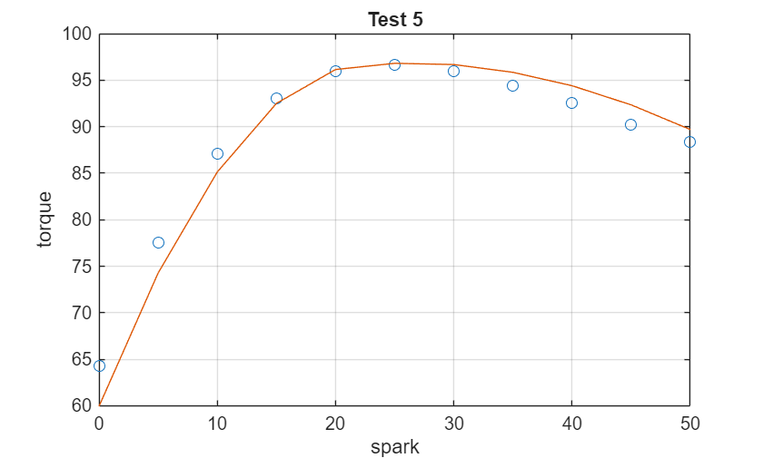
Plot the Two-stage Model of Torque Against Spark

Plot the torque versus spark for test 5.

testToPlot = 5;
BTQInputData = TQ_response.DoubleInputData(testToPlot);
BTQResponseData = TQ_response.DoubleResponseData(testToPlot);
BTQPredictedValue = TQ_response.PredictedValue( BTQInputData );
fig = figure;
plot( BTQInputData(:,1), BTQResponseData, 'o',...
BTQInputData(:,1), BTQPredictedValue, '-' );
xlabel( 'spark' );
ylabel( 'torque' );
title( 'Test 5' );
grid on

Figure contains an axes object. The axes object with title Test 5, xlabel spark, ylabel torque contains 2 objects of type line. One or more of the lines displays its values using only markers

Build Other Responses

Follow these steps to build response models for the exhaust temperature and residual fraction.

Copy outliers from torque model.
Make alternative models for each response feature.
Make a two-stage model without maximum likelihood estimation (MLE).

Exhaust Temperature Response

EXTEMP = testplan.Responses(2).LocalResponses(1);
EXTEMP.RemoveOutliers(OutlierIndices(LocalBTQ));
CreateAlternativeModels( EXTEMP,mlist, criteria );
MakeHierarchicalResponse( EXTEMP, false );
EXTEMP_RMSE = SummaryStatistics( EXTEMP, {'Local RMSE', 'Two-Stage RMSE'} )

EXTEMP_RMSE = 1×2

    10.5648    27.9918

Residual Fraction Response

RESIDFRAC = testplan.Responses(3).LocalResponses(1);
RESIDFRAC.RemoveOutliers(OutlierIndices(LocalBTQ));
CreateAlternativeModels( RESIDFRAC,mlist, criteria );
ok = MakeHierarchicalResponse( RESIDFRAC, false );
RESIDFRAC_RMSE = SummaryStatistics( RESIDFRAC, {'Local RMSE', 'Two-Stage RMSE'} )

RESIDFRAC_RMSE = 1×2

    0.0824    0.5595

if isgraphics(fig)
    % delete figure made during example
    delete(fig)
end