ODEResults
Description
ODEResults objects store the solution information from the
integration of an ode object. The solve and
solutionFcn object functions of ode can return
ODEResults objects.
You can use the Time and Solution properties of
an ODEResults object to extract or plot the integration results.
If events are being tracked (that is, the
odeobject has a nonemptyEventDefinitionproperty), then theEventTime,EventSolution, andEventIndexproperties contain information related to events that triggered during the integration. SeeodeEventfor more information on detecting events during the solution process.If sensitivity analysis is performed (that is, the
odeobject has a nonemptySensitivityproperty), then theSensitivityproperty contains partial derivative values of the equations taken with respect to parameters. If events are also being tracked, then theEventSensitivityproperty contains sensitivity values at the time of each event. SeeodeSensitivityfor more information on performing sensitivity analysis.
All properties of ODEResults objects are read-only. You can index into
the properties to extract their values with the syntax data =
obj.property.
Creation
Use solve or
solutionFcn to
integrate an ode object and
create an ODEResults object. For example, S =
solve(F,0,10) creates an ODEResults object
S.
Properties
Standard Results
This property is read-only.
Evaluation points, returned as a row vector. Typically, the independent variable in an ODE problem is time, but the independent variable can represent other quantities as well.
If you solve the ODE problem using a time range with two elements
[t0
                    tf]
, thenTimecontains the internal step values chosen by the solver.If you solve the ODE problem using a vector of times
[t0 t1 t2 ...
                    tf]
, thenTimecontains the same values.
This property is read-only.
Solution at evaluation points, returned as a matrix. Each row
Solution(i,:) is the complete solution for one component, and
each column Solution(:,j) is the solution of all components at the
corresponding evaluation point Time(j).
Event Results
This property is read-only.
Time when events triggered, returned as a row vector.
EventSolution(:,j) contains the solution of all variables at time
EventTime(j), and EventIndex(j) indicates
which event triggered.
This property is read-only.
Solution at time of events, returned as a matrix.
EventSolution has a number of columns equal to
numel(EventTime), and the same number of rows as
Solution. EventSolution(:,j) contains the
solution of all variables at time EventTime(j), and
EventIndex(j) indicates which event triggered.
This property is read-only.
Index of triggered events, returned as a row vector.
EventSolution(:,j) contains the solution of all variables at time
EventTime(j), and EventIndex(j) indicates
which event triggered.
Sensitivity Analysis
This property is read-only.
Sensitivity analysis results, returned as an array.
Sensitivity has a number of columns equal to the number of
parameters being analyzed, and the same number of rows as
Solution. The number of pages in the array is equal to the
number of time steps.
Consider an ODE system of the form
The parameters p can be treated as independent variables to
obtain the sensitivity functions
The sensitivity analysis results contain these partial derivative values of the
equations taken with respect to the parameters. You can control aspects of the
sensitivity analysis by setting properties of the odeSensitivity object assigned to the Senstivity
property of the ode object.
This property is read-only.
Sensitivity values at time of events, returned as an array.
EventSensitivity has a number of columns equal to the number of
parameters being analyzed, and the same number of rows as
Solution. The number of pages in the array is equal to the
number of events, numel(EventTime).
Examples
Create an empty ode object, and then specify values for the ODEFcn and InitialValue properties.
F = ode;
F.ODEFcn = @(t,y) 2*t;
F.InitialValue = 0;
Check which solver is selected for the problem, and then solve the equation over the time range [0 10].
F.SelectedSolver
ans =
  SolverID enumeration

    ode45
sol = solve(F,0,10)
sol =
  ODEResults with properties:

        Time: [0 0.2500 0.5000 0.7500 1 1.2500 1.5000 1.7500 2 2.2500 2.5000 2.7500 3 3.2500 3.5000 3.7500 4 4.2500 4.5000 4.7500 5 5.2500 5.5000 5.7500 6 6.2500 6.5000 6.7500 7 7.2500 7.5000 7.7500 8 8.2500 8.5000 8.7500 9 9.2500 9.5000 9.7500 10]
    Solution: [0 0.0625 0.2500 0.5625 1.0000 1.5625 2.2500 3.0625 4 5.0625 6.2500 7.5625 9 10.5625 12.2500 14.0625 16 18.0625 20.2500 22.5625 25 27.5625 30.2500 33.0625 36 39.0625 42.2500 45.5625 49 52.5625 56.2500 60.0625 64 68.0625 … ] (1×41 double)
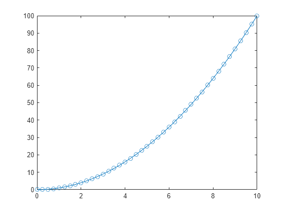
Plot the results.
plot(sol.Time,sol.Solution,"-o")
Create an ode object for the equations @(t,y) [y(2); 1000*(1-y(1)^2)*y(2)-y(1)] with the initial conditions [2 0]. Specify the solver as "stiff".
F = ode(ODEFcn=@(t,y) [y(2); 1000*(1-y(1)^2)*y(2)-y(1)],InitialValue=[2 0],Solver="stiff");Create a function handle that can evaluate the solution of the problem in the interval [0 1000] by using the solutionFcn method.
Specify
Extension="on"to enable the function handle to evaluate the solution at times outside of the original interval[0 1000].Specify
OutputVariables=1so that the function handle interpolates only the first solution variable.Specify two outputs to also return the integration results in the original interval.
[fh,S] = solutionFcn(F,0,1000,Extension="on",OutputVariables=1)fh = function_handle with value:
@ode.solutionFcn/interpolate
S =
  ODEResults with properties:

        Time: [0 1.4606e-05 2.9212e-05 4.3818e-05 1.1010e-04 1.7639e-04 2.4267e-04 3.0896e-04 4.5006e-04 5.9116e-04 7.3226e-04 8.7336e-04 0.0010 0.0012 0.0013 0.0015 0.0017 0.0018 0.0021 0.0024 0.0027 0.0030 0.0033 0.0044 0.0055 0.0066 … ] (1×227 double)
    Solution: [2×227 double]
Extract and plot the integration results for the first solution variable in S, and then use the function handle fh to also evaluate the solution in the extended interval [1000 3000]. Plot the extended solution in red.
plot(S.Time,S.Solution(1,:),"-o")
t = linspace(1000,3000);
ys = fh(t);
hold on
plot(t,ys,"r-o")
hold off

Solve an ODE system with two equations and two parameters, and perform sensitivity analysis on the parameters.
Create an ode object to represent this system of equations.
Specify the initial conditions as and , and parameter values of and . To enable sensitivity analysis of the parameters, set the Sensitivity property of the ode object to an odeSensitivity object.
p = [0.05 1.5];
F = ode(ODEFcn=@(t,y,p) [p(1)*y(1)-y(2); -p(2)*y(2)], ...
        InitialValue=[2 3], ...
        Parameters=p, ...
        Sensitivity=odeSensitivity)
F =
  ode with properties:

   Problem definition
               ODEFcn: @(t,y,p)[p(1)*y(1)-y(2);-p(2)*y(2)]
           Parameters: [0.0500 1.5000]
          InitialTime: 0
         InitialValue: [2 3]
          Sensitivity: [1×1 odeSensitivity]
         EquationType: standard

   Solver properties
    AbsoluteTolerance: 1.0000e-06
    RelativeTolerance: 1.0000e-03
               Solver: auto
       SelectedSolver: cvodesnonstiff

  Show all properties
Because the equations are nonstiff and sensitivity analysis is enabled, the ode object automatically chooses the cvodesnonstiff solver for this problem.
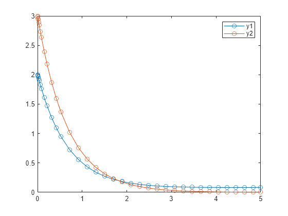
Solve the ODE over the time interval [0 5], and plot the solution for each component.
S = solve(F,0,5)
S =
  ODEResults with properties:

           Time: [0 2.9540e-09 2.9543e-05 2.2465e-04 4.1976e-04 0.0024 0.0080 0.0137 0.0245 0.0353 0.0611 0.0869 0.1499 0.2129 0.3169 0.4208 0.5248 0.7204 0.9161 1.1118 1.3075 1.5031 1.6988 1.8945 2.0901 2.2858 2.4815 2.6772 2.8728 … ] (1×40 double)
       Solution: [2×40 double]
    Sensitivity: [2×2×40 double]
plot(S.Time,S.Solution(1,:),"-o",S.Time,S.Solution(2,:),"-o")
legend("y1","y2")

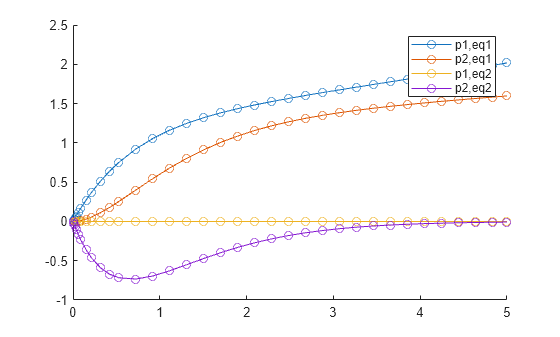
The values in S.Sensitivity are partial derivatives of the equations with respect to the parameters. To examine the effects of the parameter values during the integration, plot the sensitivity values.
figure
hold on
plot(S.Time,squeeze(S.Sensitivity(1,1,:)),"-o")
plot(S.Time,squeeze(S.Sensitivity(1,2,:)),"-o")
plot(S.Time,squeeze(S.Sensitivity(2,1,:)),"-o")
plot(S.Time,squeeze(S.Sensitivity(2,2,:)),"-o")
legend("p1,eq1","p2,eq1","p1,eq2","p2,eq2")
hold off

Consider a ball thrown upward with an initial velocity . The ball is subject to acceleration due to gravity aimed downward, so its acceleration is
Rewriting the equation as a first-order system of equations with the substitutions and yields
Solve the equations for the position and velocity of the ball over time.
Define Equations and Initial Conditions
Create a function handle for the first-order system of equations that accepts two inputs for (t,y). Use the value for the acceleration due to gravity.
dydt = @(t,y) [y(2); -9.8];
Next, create a vector with the initial conditions. The ball starts at position at as it is thrown upward with initial velocity .
y0 = [3 20];
Model Ball Bounces as Events
The ball initially travels upward until the force due to gravity causes it to change direction and head back down to the ground. If you solve the equations without more consideration, then the ball falls back downward forever without striking the ground. Instead, you can use an event function to detect when the position of the ball goes to zero where the ground is located. Because the solution component is the position of the ball, the event function tracks the value of so that an event triggers whenever .
Create a function handle for the event function that accepts two inputs for (t,y).
bounceEvent = @(t,y) y(1);
When the ball strikes the ground, its direction changes again as it heads back upwards with a new (smaller) initial velocity. To model this situation, use a callback function along with the event function. When an event triggers, the ODE solver invokes the callback function. The callback function resets the position and initial velocity of the ball so that the integration can restart with the correct initial conditions. When an event occurs, the callback function sets the position and attenuates the velocity by a factor of while reversing its direction back upward. Define a callback function that performs these actions.
function [stop,y] = bounceResponse(t,y)
stop = false;
y(1) = 0;
y(2) = -0.9*y(2);
end
(The callback function is included as a local function at the end of the example.)
Create an odeEvent object to represent the bouncing ball events. Specify Direction="descending" so that only events where the position is decreasing are detected. Also, specify Response="callback" so that the solver invokes the callback function when an event occurs.
E = odeEvent(EventFcn=bounceEvent, ...
             Direction="descending", ...
             Response="callback", ...
             CallbackFcn=@bounceResponse)
E =
  odeEvent with properties:

       EventFcn: @(t,y)y(1)
      Direction: descending
       Response: callback
    CallbackFcn: @bounceResponse
Solve Equations
Create an ode object for the problem, specifying the equations dydt, initial conditions y0, and events E as property values.
F = ode(ODEFcn=dydt,InitialValue=y0,EventDefinition=E);
Integrate the equations over the time interval [0 30] by using the solve method. Specify Refine=8 to generate 8 points per step. The resulting object has properties for the time and solution, and because events are being tracked, the object also displays properties related to the events that triggered during the integration.
S = solve(F,0,30,Refine=8)
S =
  ODEResults with properties:

             Time: [0 0.0038 0.0075 0.0113 0.0151 0.0188 0.0226 0.0264 0.0301 0.0490 0.0678 0.0867 0.1055 0.1243 0.1432 0.1620 0.1809 0.2751 0.3692 0.4634 0.5576 0.6518 0.7460 0.8402 0.9344 1.3094 1.6844 2.0594 2.4344 2.8094 3.1844 … ] (1×468 double)
         Solution: [2×468 double]
        EventTime: [4.2265 8.1607 11.7015 14.8882 17.7563 20.3375 22.6606 24.7514 26.6331 28.3267 29.8509]
    EventSolution: [2×11 double]
       EventIndex: [1 1 1 1 1 1 1 1 1 1 1]
Plot Results
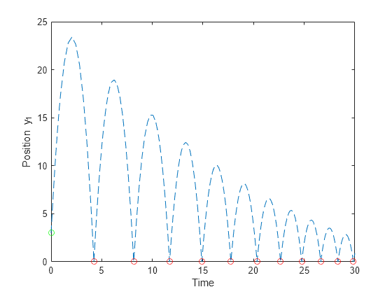
Plot the position of the ball over time, marking the initial position with a green circle and events with red circles.
plot(S.Time,S.Solution(1,:),"--")
hold on
plot(S.EventTime,S.EventSolution(1,:),"ro")
plot(0,y0(1),"go")
hold off
ylim([0 25])
xlabel("Time")
ylabel("Position y_1")

Local Functions
function [stop,y] = bounceResponse(t,y)
stop = false;
y(1) = 0;
y(2) = -0.9*y(2);
end
Version History
Introduced in R2023b
See Also
ode | odeEvent | odeSensitivity | solve | solutionFcn
MATLAB Command
You clicked a link that corresponds to this MATLAB command:
Run the command by entering it in the MATLAB Command Window. Web browsers do not support MATLAB commands.
웹사이트 선택
번역된 콘텐츠를 보고 지역별 이벤트와 혜택을 살펴보려면 웹사이트를 선택하십시오. 현재 계신 지역에 따라 다음 웹사이트를 권장합니다:
또한 다음 목록에서 웹사이트를 선택하실 수도 있습니다.
사이트 성능 최적화 방법
최고의 사이트 성능을 위해 중국 사이트(중국어 또는 영어)를 선택하십시오. 현재 계신 지역에서는 다른 국가의 MathWorks 사이트 방문이 최적화되지 않았습니다.
미주
- América Latina (Español)
- Canada (English)
- United States (English)
유럽
- Belgium (English)
- Denmark (English)
- Deutschland (Deutsch)
- España (Español)
- Finland (English)
- France (Français)
- Ireland (English)
- Italia (Italiano)
- Luxembourg (English)
- Netherlands (English)
- Norway (English)
- Österreich (Deutsch)
- Portugal (English)
- Sweden (English)
- Switzerland
- United Kingdom (English)