미국 인구 예측(Predicting the US Population)

이 예제에서는 차수가 높은 다항식을 사용하여 데이터를 외삽하는 것이 위험하고 신뢰할 수 없음을 보여줍니다.

이 예제는 MATLAB®이 출시되기 이전부터 사용되었습니다. 이 예제는 1977년에 Prentice-Hall에서 출판한 Computer Methods for Mathematical Computations(저자: Forsythe, Malcolm, Moler)에 연습 과제로 처음 소개되었습니다.

이제는 MATLAB을 통해 파라미터에 변화를 주고 결과를 확인하는 것이 훨씬 더 쉬워졌지만 기본적인 수학 원리는 변하지 않았습니다.

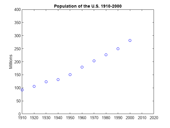
1910년부터 2000년까지의 미국 인구 조사 데이터로 2개의 벡터를 만들고 플로팅해 보겠습니다.

% Time interval
t = (1910:10:2000)';

% Population
p = [91.972 105.711 123.203 131.669 150.697...
    179.323 203.212 226.505 249.633 281.422]';

% Plot
plot(t,p,'bo');
axis([1910 2020 0 400]);
title('Population of the US 1910-2000');
ylabel('Millions');

Figure contains an axes object. The axes object with title Population of the US 1910-2000, ylabel Millions contains a line object which displays its values using only markers.

2010년도의 인구는 어느 정도나 될 것으로 추측됩니까?

t에 관한 다항식으로 데이터를 피팅하고 이를 사용하여 t = 2010일 때 인구를 외삽합니다. 11×11 크기의 방데르몽드 행렬을 포함하는 선형 연립방정식을 풀어 다항식의 계수를 구합니다. 이 행렬의 요소는 A(i,j) = s(i)^(n-j)로서, 스케일링된 시간의 거듭제곱입니다.

n = length(t);
s = (t-1950)/50;
A = zeros(n);
A(:,end) = 1;
for j = n-1:-1:1
   A(:,j) = s .* A(:,j+1);
end

방데르몽드 행렬의 마지막 d+1개 열을 포함하는 다음 선형 연립방정식을 풀어 데이터 p를 피팅하는, 차수가 d인 다항식의 계수 c를 구합니다.

A(:,n-d:n)*c ~= p

d < 10이면, 미지수보다 방정식이 더 많은 경우가 되므로 최소제곱해가 적절합니다.
d == 10이면, 방정식의 완전한 해를 구할 수 있으며 다항식은 실제로 데이터를 보간합니다.

두 경우 모두 백슬래시 연산자를 사용하여 시스템을 풀 수 있습니다. 다음은 3차 피팅의 계수입니다.

c = A(:,n-3:n)\p

이제 1910년부터 2010년까지 매년 다항식을 계산하고 결과를 플로팅해 보겠습니다.

v = (1910:2020)';
x = (v-1950)/50;
w = (2010-1950)/50;
y = polyval(c,x);
z = polyval(c,w);

hold on
plot(v,y,'k-');
plot(2010,z,'ks');
text(2010,z+15,num2str(z));
hold off

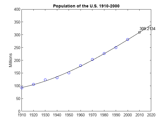
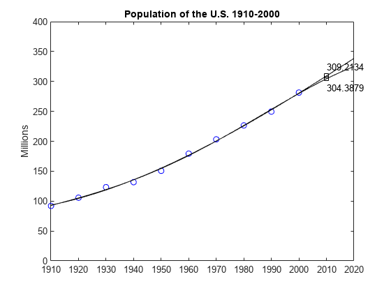
Figure contains an axes object. The axes object with title Population of the US 1910-2000, ylabel Millions contains 4 objects of type line, text. One or more of the lines displays its values using only markers

3차 피팅과 4차 피팅을 비교해 보면 외삽 지점이 매우 다른 것을 알 수 있습니다.

c = A(:,n-4:n)\p;
y = polyval(c,x);
z = polyval(c,w);

hold on
plot(v,y,'k-');
plot(2010,z,'ks');
text(2010,z-15,num2str(z));
hold off

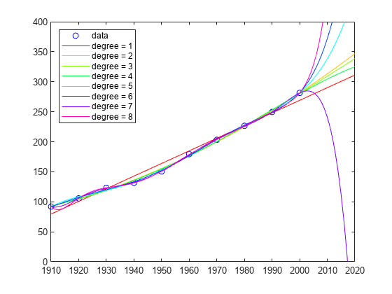
Figure contains an axes object. The axes object with title Population of the US 1910-2000, ylabel Millions contains 7 objects of type line, text. One or more of the lines displays its values using only markers

차수가 증가할수록 외삽의 오차가 오히려 커집니다.

cla
plot(t,p,'bo')
hold on
axis([1910 2020 0 400])
colors = hsv(8);
labels = {'data'};
for d = 1:8
   [Q,R] = qr(A(:,n-d:n));
   R = R(1:d+1,:);
   Q = Q(:,1:d+1);
   c = R\(Q'*p);    % Same as c = A(:,n-d:n)\p;
   y = polyval(c,x);
   z = polyval(c,w);
   plot(v,y,'color',colors(d,:));
   plot(2010,z,'s','color',colors(d,:));
   labels{end+1} = ['degree = ' int2str(d)];
   labels{end+1} = '';
end
legend(labels, 'Location', 'NorthWest')
hold off

Figure contains an axes object. The axes object contains 17 objects of type line. One or more of the lines displays its values using only markers These objects represent data, degree = 1, degree = 2, degree = 3, degree = 4, degree = 5, degree = 6, degree = 7, degree = 8.

참고 항목

polyfit