이 페이지는 기계 번역을 사용하여 번역되었습니다. 영어 원문을 보려면 여기를 클릭하십시오.
스펙트럼 분석기 그래프
이 예제는 Quick Control Spectrum Analyzer를 사용하여 Keysight® Technologies N9040B 스펙트럼 분석기에서 파워 스펙트럼 데이터를 수집하는 방법을 보여줍니다.
소개
이 예제에서는 스펙트럼 분석기를 사용하여 2.402 GHz에서 2.48 GHz 사이의 Bluetooth® 대역 내에서 파워 스펙트럼 데이터를 수집합니다.
요구 사항
이 예제를 실행하려면 다음이 필요합니다.
Keysight 테크놀로지스 N9040B 스펙트럼 분석기
Keysight 테크놀로지스 N9040B 스펙트럼 분석기용 IVI-C 드라이버 (AgXSAn)
NI™ VISA 또는 Keysight VISA
NI IVI® 규정 준수 패키지 버전 16.0.1.2 이상
RF 스펙트럼 분석기 객체 생성
Quick Control 객체를 생성하고 사용 가능한 리소스와 드라이버를 검색합니다.
rfsa = rfspecan;
resources(rfsa)
ans =
    ' TCPIP0::K-N9040B-91124.dhcp.mathworks.com::inst0::INSTR
     '
drivers(rfsa)
ans =
    'Driver: AgXSAn
     Supported Models:
        M8920A, M90XA, M9290A, M9410A, M9411A, M9415A, M9420A
        M9421A, N8973B, N8974B, N8975B, N8976B, N9000A, N9000B
        N9010A, N9010B, N9020A, N9020B, N9021B, N9030A, N9030B
        N9032B, N9038A, N9038B, N9040B, N9041B, N9042B, N9048B

     Driver: rsspecan
     Supported Models:
     ESW, FPH, FPS, FSV, FSVA, FSVR, FSW, FSWP, FSWT

     '
선택한 리소스 및 드라이버에 연결
사용 가능한 리소스와 드라이버를 선택하십시오.
rfsa.Resource = "TCPIP0::K-N9040B-91124.dhcp.mathworks.com::inst0::INSTR";
rfsa.Driver = "AgXSAn";
connect(rfsa)
disp(rfsa)
  RFSpecAn with properties:

                Resource: "TCPIP0::K-N9040B-91124.dhcp.mathworks.com::inst0::INSTR"
                  Driver: "AgXSAn"
                  Vendor: "Keysight Technologies"
                   Model: "N9040B"
          StartFrequency: 10000000
           StopFrequency: 2.6500e+10
         CenterFrequency: 1.3255e+10
                    Span: 2.6490e+10
               SweepTime: 0.0665
     ResolutionBandwidth: 3000000
          VideoBandwidth: 3000000
           VerticalScale: Logarithmic
          AmplitudeUnits: dBm
          ReferenceLevel: 0
    ReferenceLevelOffset: 0

  Show all properties, functions
시작 및 정지 주파수 설정
시작 주파수를 2.402 GHz인 블루투스 대역의 시작 지점 바로 아래로 설정하십시오. 정지 주파수를 2.48 GHz인 블루투스 대역의 끝 지점 바로 위로 설정하십시오.
rfsa.StartFrequency = 2.4e9;
rfsa.StopFrequency = 2.5e9
  RFSpecAn with properties:

                Resource: "TCPIP0::K-N9040B-91124.dhcp.mathworks.com::inst0::INSTR"
                  Driver: "AgXSAn"
                  Vendor: "Keysight Technologies"
                   Model: "N9040B"
          StartFrequency: 2.4000e+09
           StopFrequency: 2.5000e+09
         CenterFrequency: 2.4500e+09
                    Span: 100000000
               SweepTime: 1.0000e-03
     ResolutionBandwidth: 910000
          VideoBandwidth: 910000
           VerticalScale: Logarithmic
          AmplitudeUnits: dBm
          ReferenceLevel: 0
    ReferenceLevelOffset: 0

  Show all properties, functions
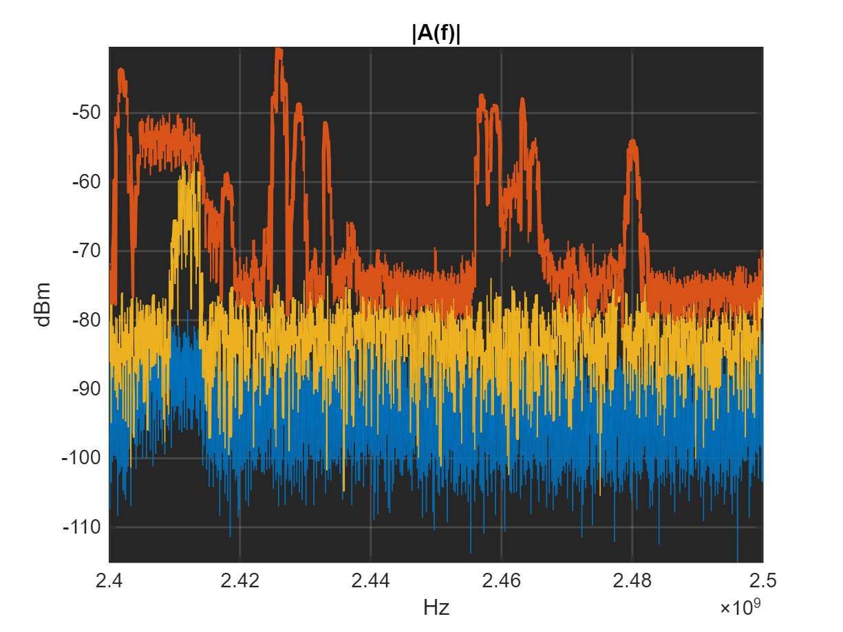
파워 스펙트럼 진폭 데이터 수집
실수 값을 갖는 파워 스펙트럼 100개를 수집하십시오. 각 스펙트럼에는 TraceSize와 동일한 수의 데이터 포인트가 포함되며, TraceSize는 N9040B에서 고정된 값입니다.
n = 100;
data = nan(rfsa.TraceSize, n);
for i = 1:n
    data(:, i) = readPowerSpectrum(rfsa);
end
수집된 데이터의 평균과 엔벨로프를 그래프로 표시하십시오
이는 사실상 “최소 홀드(Minimum Hold)” 및 “최대 홀드(Maximum Hold)” 추적 유형을 사용하여 데이터를 수집하는 것과 동일합니다.
Amin = min(data, [], 2);
Amax = max(data, [], 2);
Amean = mean(data, 2);

f = linspace(rfsa.StartFrequency, rfsa.StopFrequency, rfsa.TraceSize);

figure;
hold on

plot(f, Amin, LineWidth=2);
plot(f, Amax, LineWidth=2);
plot(f, Amean, LineWidth=2);

title("|A(f)|")
% Label using the current units of amplitude, which are set to "dBm" by
% default.
ylabel(string(rfsa.AmplitudeUnits));
xlabel("Hz")

setAxesSpectrumAnalyzer(gca);

현재 데이터를 실시간으로 그래프에 표시하고 최대값 및 최소값을 추적합니다
전면 패널 디스플레이에 관측된 데이터를 세 개의 파형(샘플, 최소값, 최대값)으로 표시합니다.
figure;

Amin = data(:, 1);
Amax = data(:, 1);
Anext = data(:, 1);

p = plot(f, Amin, f, Anext, f, Amax, LineWidth=2);
ax = gca;
setAxesSpectrumAnalyzer(ax)
colors = colororder;
order = [1 3 2];
ax.ColorOrder = colors(order, :);

title("|A(f)|")
ylabel(string(rfsa.AmplitudeUnits));
xlabel("Hz")

axis tight

p(1).YDataSource =  'Amin';
p(2).YDataSource =  'Anext';
p(3).YDataSource =  'Amax';

for i = 2:n
    Anext = data(:, i);
    Amin = min(Amin, Anext);
    Amax = max(Amax, Anext);

    axis tight
    refreshdata
    drawnow limitrate nocallbacks
    pause(0.100);
end
전면 패널 디스플레이
function setAxesSpectrumAnalyzer(haxes)
% Configure the plot to look like a front-panel display
% of a stand-alone instrument.

set(haxes, 'Color', [0.150 0.150 0.150], ...
           'GridColor', [1 1 1], ...
           'GridLineWidth', 1, ...
           'XGrid','on', ...
           'YGrid','on');
end