mtf
R2026bDescription
Add-On Required: This feature requires the Optical Design and Simulation Library for Image Processing Toolbox add-on.
computes the modulation transfer function (MTF) for the optical system
mtfr = mtf(opsys)opsys using the default field points and wavelengths. The MTF
represents contrast transfer as a function of spatial frequency in the image plane. The
function computes MTF from a PSF generated for the specified field points and
wavelengths.
specifies options using one or more name-value arguments. For example,
mtfr = mtf(opsys,Name=Value)mtf(opsys,FieldPoints=fp,Wavelengths=587.56,Method="Huygens")
computes a wave-optics MTF for the field point fp at a wavelength of
587.56 nanometers. The function uses these options to generate the PSF from which it
computes the MTF.
Examples
Load the sample Double Gauss lens system using zmximport. Define an off-axis field point at an angle of 3 degrees along the y-axis, and compute the geometric MTF for three distinct wavelengths (486.1 nm, 587.6 nm, and 656.3 nm).
opsys = zmximport("DoubleGaussLens.zmx");
fp = fieldPoint(Angles=[0 3]);
mtfr = mtf(opsys, FieldPoints=fp, Wavelengths=[486.1 587.6 656.3])mtfr =
GeometricMTF with properties:
Tangential: [1×1 struct]
Sagittal: [1×1 struct]
FieldPoint: [1×1 optics.fieldpoint.FieldAngle]
Wavelengths: [486.1000 587.6000 656.3000]
FFTLength: [128 128]
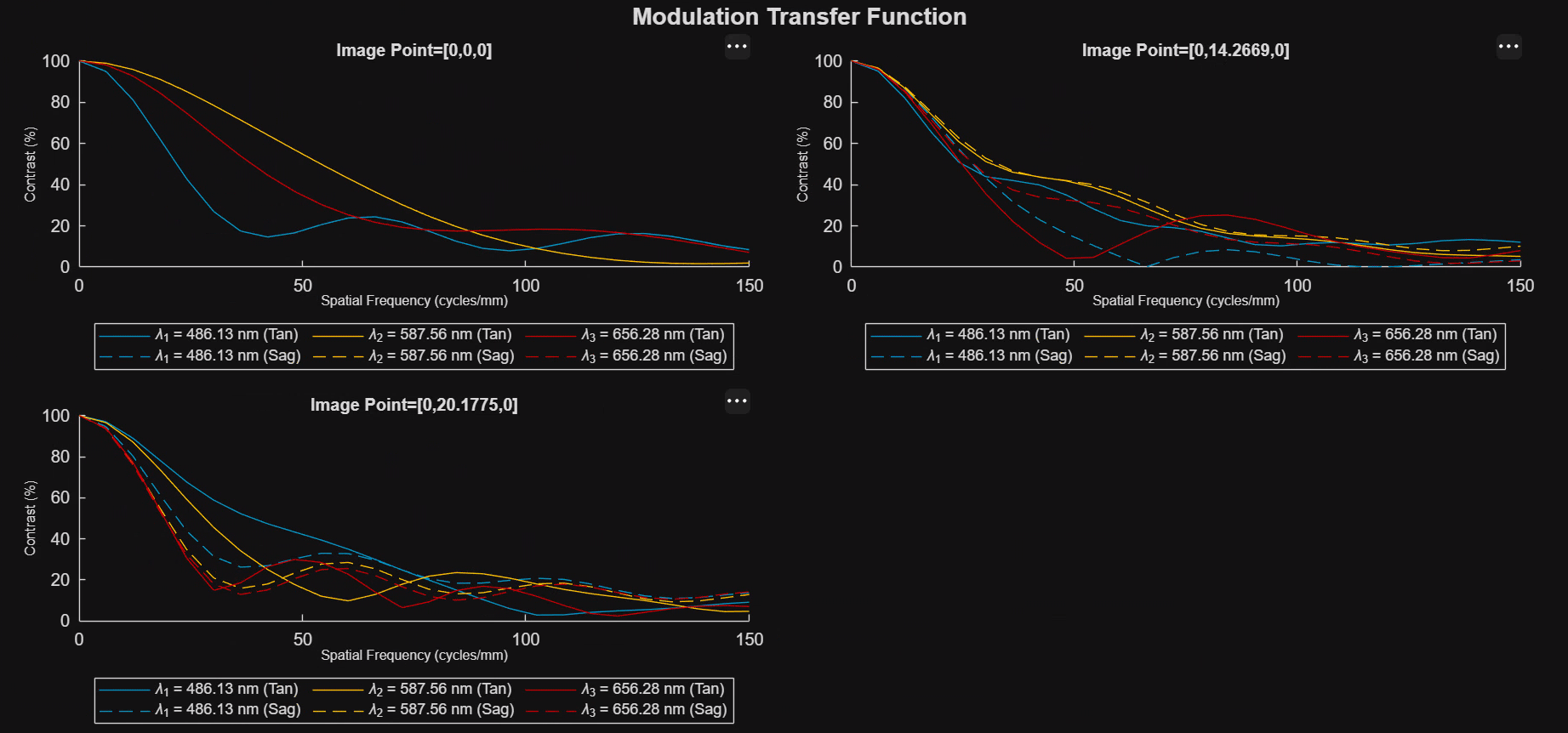
Load the sample Double Gauss lens system using zmximport. Compute the Huygens MTF by setting the Method name-value argument to "Huygens". Limit the output curves to a spatial frequency of 150 cycles per millimeter using the MaximumFrequency argument, and specify an FFTLength of 512 to achieve higher frequency resolution.
opsys = zmximport("DoubleGaussLens.zmx"); mtfr = mtf(opsys, Method="Huygens", MaximumFrequency=150, FFTLength=512);
Visualize the tangential and sagittal contrast curves as a function of spatial frequency by passing the result object to the show function.
hmtf = show(mtfr)
hmtf =
MTFChart with properties:
Legend: on
Grid: "off"
Title: "Modulation Transfer Function"
MTF: [1×3 optics.result.HuygensMTF]
WavelengthIndices: [1 2 3]
Color: [3×3 double]
Position: [0.0737 0.2521 0.8713 0.5977]
Units: 'normalized'
Show all properties
Load the sample Double Gauss lens system using zmximport. Compute the geometric MTF up to a maximum spatial frequency of 200 cycles per millimeter by setting the MaximumFrequency name-value argument.
opsys = zmximport("DoubleGaussLens.zmx");
mtfr = mtf(opsys, MaximumFrequency=200);Use the frequencyAtContrast function to compute MTF50, the spatial frequency where the MTF first drops to 50% contrast. Then, use the contrastAtFrequency function to determine the exact sagittal and tangential contrast values at spatial frequencies of 30, 60, and 100 cycles per millimeter.
By default, these functions evaluate the entire optical system simultaneously and return multi-dimensional arrays. The dimensions map to [Fields, Wavelengths, Configurations, Planes] for the MTF50 output, and [Fields, Wavelengths, Frequencies, Planes] for the contrast output, where the rows represent field points and the columns represent wavelengths.
MTF50 = frequencyAtContrast(mtfr, 0.5)
MTF50 = MTF50(:,:,1,1) = 22.2302 48.5808 37.1994 30.4516 44.1749 35.1107 26.2930 20.7316 19.6589 MTF50(:,:,1,2) = 22.2300 48.5906 37.2039 31.2080 43.8519 27.4440 52.5096 33.6761 18.1949
contrast = contrastAtFrequency(mtfr, [30; 60; 100])
contrast =
contrast(:,:,1,1) =
0.4014 0.7605 0.6261
0.5084 0.6298 0.5519
0.4752 0.3834 0.3539
contrast(:,:,2,1) =
0.2572 0.3637 0.2569
0.1174 0.3793 0.2909
0.3216 0.2569 0.2353
contrast(:,:,3,1) =
0.1793 0.0742 0.2620
0.0475 0.1648 0.0820
0.2108 0.1898 0.1699
contrast(:,:,1,2) =
0.4014 0.7606 0.6262
0.5081 0.6205 0.4417
0.7480 0.5750 0.3493
contrast(:,:,2,2) =
0.2572 0.3639 0.2569
0.2959 0.3558 0.1313
0.4327 0.2412 0.2650
contrast(:,:,3,2) =
0.1793 0.0742 0.2618
0.0944 0.1362 0.1943
0.0866 0.2809 0.2394
Input Arguments
Optical system for which to compute the modulation transfer function, specified as
an opticalSystem object.
Name-Value Arguments
Specify optional pairs of arguments as
Name1=Value1,...,NameN=ValueN, where Name is
the argument name and Value is the corresponding value.
Name-value arguments must appear after other arguments, but the order of the
pairs does not matter.
Example: mtf(opsys,Method="Huygens",MaximumFrequency=150,FFTLength=512)
computes a wave-optics MTF up to 150 cycles per millimeter using an FFT length of 512.
Field points for the MTF computation, specified as a FieldAngle
object, a FieldPosition object, or an array of field point objects. Each returned
mtfr element contains the MTF for one field point.
By default, the FieldPoints value is the
FieldPoints property of opsys.
Wavelengths for MTF computation, specified as an M-element numeric vector. M is the number of wavelengths, and each element of the vector is a wavelength in nanometers. The returned MTF object contains tangential and sagittal curves for each specified wavelength.
Data Types: double
MTF computation method, specified as "Geometric" or
"Huygens". This argument controls the internal PSF computation
used to compute the MTF and the type of MTF result object returned.
| Method | Description |
|---|---|
"Geometric" | Compute the MTF from a geometric PSF. Use this method for fast analysis when aberrations are large compared to diffraction-limited performance. |
"Huygens" | Compute the MTF from a Huygens PSF. Use this method when diffraction and phase effects are important. |
Index of the reference wavelength, specified as a positive integer. The reference wavelength is used to determine the chief ray hit position for centering the internal PSF used to compute the MTF.
If you specify Wavelengths and do not specify
ReferenceWavelengthIndex, the function uses the index of the
median wavelength after sorting the wavelength values. If you do not specify
Wavelengths, the reference wavelength is specified by the
PrimaryWavelengthIndex property of opsys.
Maximum spatial frequency for the MTF curves, specified as a nonnegative scalar
in cycles per millimeter. The function evaluates the tangential and sagittal MTF
curves on a frequency grid from 0 to MaximumFrequency.
By default, the function uses the diffraction-limited cutoff frequency
1/(lambda*FNumber) at the primary wavelength.
Data Types: double
FFT size for computing the optical transfer function from the internal PSF, specified as a positive integer scalar or a 1-by-2 vector of positive integers. If you specify a scalar, the function uses the same FFT length for rows and columns. If you specify a vector, the first element is the number of rows and the second element is the number of columns.
The value of FFTLength must be greater than or equal to
PSFResolution in each dimension. Larger values provide denser
frequency sampling but do not change the maximum frequency.
Data Types: double
Resolution of the internal PSF image used to compute the MTF, specified as a 1-by-2 vector of positive integers of the form [width height].
Spatial sampling interval of the internal PSF image in the image plane, specified as a positive scalar in microns. The internal PSF pixel size determines the spatial sampling used before the Fourier transform.
Data Types: double
Output Arguments
Modulation transfer function results, returned as an array of
optics.result.GeometricMTF objects when Method
is "Geometric", or an array of
optics.result.HuygensMTF objects when Method is
"Huygens". The returned array contains one object for each field
point specified by FieldPoints.
Each MTF object contains Tangential and
Sagittal structures for the specified wavelengths. Each structure
contains spatial frequency values in cycles per millimeter and corresponding MTF
values.
The MTF result objects expose the Tangential,
Sagittal, FieldPoint,
Wavelengths, and FFTLength properties.
More About
The modulation transfer function describes how an optical system transfers image contrast at different spatial frequencies. Higher MTF values indicate better contrast transfer at the corresponding spatial frequency.
The mtf function computes separate tangential and sagittal
curves so you can compare contrast transfer along the principal image-plane directions.
The mtf function computes the MTF from an internal point
spread function (PSF). A narrower PSF generally corresponds to slower MTF rolloff and better
contrast transfer at higher spatial frequencies.
The mtf function computes MTF from the PSF of the optical
system using Fourier analysis. The MTF describes contrast transfer as a function of spatial
frequency and is returned separately for sagittal and tangential directions.
Version History
Introduced in R2026b
See Also
psf | airyDiskRadius | GeometricMTF | HuygensMTF | contrastAtFrequency | frequencyAtContrast | spot | opticalSystem | fieldPoint | MTFChart
MATLAB Command
You clicked a link that corresponds to this MATLAB command:
Run the command by entering it in the MATLAB Command Window. Web browsers do not support MATLAB commands.
웹사이트 선택
번역된 콘텐츠를 보고 지역별 이벤트와 혜택을 살펴보려면 웹사이트를 선택하십시오. 현재 계신 지역에 따라 다음 웹사이트를 권장합니다:
또한 다음 목록에서 웹사이트를 선택하실 수도 있습니다.
사이트 성능 최적화 방법
최고의 사이트 성능을 위해 중국 사이트(중국어 또는 영어)를 선택하십시오. 현재 계신 지역에서는 다른 국가의 MathWorks 사이트 방문이 최적화되지 않았습니다.
미주
- América Latina (Español)
- Canada (English)
- United States (English)
유럽
- Belgium (English)
- Denmark (English)
- Deutschland (Deutsch)
- España (Español)
- Finland (English)
- France (Français)
- Ireland (English)
- Italia (Italiano)
- Luxembourg (English)
- Netherlands (English)
- Norway (English)
- Österreich (Deutsch)
- Portugal (English)
- Sweden (English)
- Switzerland
- United Kingdom (English)