Improve Manufacturing Yield Using Monte Carlo Analysis

R2026b

Since R2026b

This example demonstrates how to use Monte Carlo simulation to evaluate and improve the manufacturing yield of an optical system. Manufacturing yield is the percentage of fabricated lenses that meet a target image quality specification after accounting for random variations in surface radii, element thicknesses, air gaps, and glass properties that occur during production. A high yield indicates fewer rejected lenses and lower per-unit cost.

In this example, you perform these steps.

1. Run direct sensitivity analysis on the optical system to identify the worst offenders, that is, the parameters that have the largest negative impact on the yield.

2. Run Monte Carlo simulation to measure baseline yield.

3. Tighten, that is, reduce the tolerances of the worst offenders, and widen the range of the compensator.

4. Rerun the Monte Carlo simulation to confirm the improved yield.

This example requires the Optical Design and Simulation Library for Image Processing Toolbox™ and the Optimization Toolbox™. The compensator uses the Optimization Toolbox during sensitivity analysis and Monte Carlo trials to optimize the position of the image plane. You can install the Optical Design and Simulation Library for Image Processing Toolbox from the Add-On Explorer. For more information about installing add-ons, see Get and Manage Add-Ons.

If the Parallel Computing Toolbox™ is available, Monte Carlo trials run in parallel on a local cluster for faster execution. Without the Parallel Computing Toolbox, the Monte Carlo trials run sequentially.

Import Cooke Triplet

The five Seidel aberrations are the primary defects that degrade image quality in optical systems. Specifically, the Seidel aberrations are spherical aberration, coma, astigmatism, field curvature, and distortion. The Cooke triplet is a three-element lens design that corrects the Seidel aberrations. Import the Cooke triplet optical system from a ZMX file, using the zmximport function, and visualize the optical system.

opsys = zmximport("CookeTriplet.zmx");
view2d(opsys)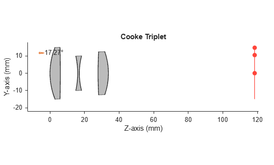

ans = 
  OpticalSystemViewer2D with properties:

            Title: ""
    OpticalSystem: [1×1 opticalSystem]
           Labels: "none"
      FieldPoints: "on"
             Rays: [0×0 optics.ui.Rays2D]
           Parent: [1×1 Figure]

  Show all properties

Specify the design wavelengths as the standard F (486.1 nm), d (587.6 nm), and C (656.3 nm) Fraunhofer lines spanning the visible spectrum. Define three field points, at 0, 5, and 7 degrees either in the horizontal or vertical direction, to capture different aberration sensitivities across the field. Focus the optical system at the mid-field point to balance on-axis and full-field performance.

opsys.Wavelengths = [486.1 587.6 656.3];
opsys.FieldPoints = fieldPoint(Angles=[0 0;0 5;7 0]);
focus(opsys,FieldPoint=opsys.FieldPoints(2),Wavelengths=opsys.Wavelengths);

Define Merit Function and Compensator

Define an optical merit function that evaluates the root mean square (RMS) spot size, which measures how tightly traced rays converge at the image plane. The merit function evaluates the spot size across all field points and wavelengths and returns a composite score. By default, the addSpot function uses all field points and wavelengths defined in the optical system to evaluate the spot size.

meritFcn = opticalMeritFunction;
meritFcn = addSpot(meritFcn)

meritFcn = 
  opticalMeritFunction with properties:

         Metrics: [1×1 optics.metric.SpotRMS]
         Weights: 1
    MetricsTable: [1×4 table]

Define a compensator that models the back-focus adjustment available during assembly. Image planes typically have a mechanical adjustment knob that enables you to shift the position of the detector along the optical axis. Because the Cooke triplet optical system has an image plane as its last component, you can add a compensator that moves the image plane within +/-0.5 mm along the Z-axis, which is the optical axis. During each sensitivity evaluation, the compensator moves the image plane within the permitted +/-0.5 mm range to the position that minimizes the merit function, so that reported contributions reflect the best achievable performance after focus adjustment.

numComponents = numel(opsys.Components);

% Verify the system ends with an image plane (required for this compensator)
assert(isa(opsys.Components(end),"optics.component.ImagePlane"), ...
    "Last component must be an ImagePlane. " + ...
    "If using your own system, add an image plane with addImagePlane.");

compSet = opticalOptimizationSet;
compSet = addComponentPositionTuning(compSet,PositionZ=[-0.5 0.5],TargetIndex=numComponents);

Define Initial Tolerances

Define initial tolerances based on fabrication experience and manufacturer specifications. The initial tolerances represent the starting point for the iterative tolerancing process. The primary performance drivers for a Cooke triplet are the surface radius, the component thickness, the air gap, and the material properties such as refractive index and Abbe number.

Define tolerances for the surface radius by adding surface radius tolerances for all the curved surfaces, with a range of +/-0.1 mm, which is a typical test plate fit tolerance.

tolSet = opticalToleranceSet;
tolSet = addSurfaceRadiusTolerance(tolSet,[-0.1 0.1]);

Define tolerances for the component thickness by adding surface position tolerances for the terminating surfaces of each lens, with a range of +/-0.05 mm.

tolSet = addSurfacePositionTolerance(tolSet,PositionZ=[-0.05 0.05],TargetIndex=[2 4 6]);

Define tolerances for the air gap by adding component position tolerances for each lens, with a range of +/-0.08 mm.

numLensElements = numComponents-1;
tolSet = addComponentPositionTolerance(tolSet,PositionZ=[-0.08 0.08],TargetIndex=1:numLensElements);

Material tolerances account for melt-to-melt variation in glass properties. Refractive index (Nd) varies by approximately +/-0.0005 between melts of the same glass type for standard-grade glass, and Abbe number (Vd) varies by approximately +/-0.5. These values are representative starting points and actual tolerances depend on the glass type and supplier grade selected for production. Define tolerances for the material of components by adding tolerances for the refractive index (Nd) and Abbe number (Vd) of the component materials.

tolSet = addComponentMaterialTolerance(tolSet,Nd=[-0.0005 0.0005]);
tolSet = addComponentMaterialTolerance(tolSet,Vd=[-0.5 0.5]);

Run Forward Sensitivity Analysis

Run a sensitivity analysis, using the opticalSensitivity object function of the opticalSystem object, to identify the parameters that are the worst offenders. The opticalSensitivity function perturbs each parameter once to its upper tolerance bound and once to its lower tolerance bound, optimizes the compensator, and records the worst-case spot size degradation. This analysis shows which parameters have the largest impact on the performance of the optical system at their current tolerance values.

sensResult = opticalSensitivity(opsys,meritFcn,tolSet,Compensator=compSet,UseParallel=true);
nominalVal = sensResult.NominalMeritValue;
tbl = sensResult.ResultTable;
numTol = height(tbl);

For each parameter, compute the worst-case contribution, that is, the maximum absolute deviation from the nominal value out of both perturbation bounds.

paramNames = tbl.TargetProperty;
targetIndices = tbl.TargetIndex;
paramTypes = tbl.TargetPropertyType;

contributions = zeros(numTol, 1);
for idx = 1:numTol
    scores = tbl.MetricScore{idx};
    contributions(idx) = max(abs(scores{1} - nominalVal),abs(scores{2} - nominalVal));
end

To create display labels for each tolerance parameter, use the buildParameterLabels supporting function, which is defined at the end of this example.

labels = buildParameterLabels(paramNames,paramTypes,targetIndices);

Identify Worst Offenders

Sort parameters by their contribution to spot size degradation. The contribution column shows how much each parameter degrades RMS spot size, in mm, when perturbed to its tolerance bound. Parameters with the largest contributions are the best candidates for tightening, that is, shrinking their tolerances. Tightening only the top five worst offenders, that is, the five parameters with the largest contributions to RMS spot size, has a much greater impact on yield than uniformly tightening all parameters.

[sortedContrib, worstIdx] = sort(contributions,"descend");

numWorst = min(5, numel(worstIdx));
worstLabels = labels(worstIdx(1:numWorst));
worstContribValues = sortedContrib(1:numWorst);

sensitivityTbl = table(worstLabels,worstContribValues,VariableNames=["Parameter","Contribution (mm RMS)"]);
disp("Top 5 worst offenders (largest impact on spot size):");

Top 5 worst offenders (largest impact on spot size):

disp(sensitivityTbl);

             Parameter             Contribution (mm RMS)
    ___________________________    _____________________

    "Radius (Surface 6)"                 0.0012554      
    "Abbe Number (Component 2)"          0.0010178      
    "Radius (Surface 4)"                 0.0007872      
    "Radius (Surface 3)"                0.00072705      
    "Radius (Surface 1)"                0.00070345      

Perform Baseline Tolerancing

To establish the baseline yield, run 100 Monte Carlo trials with the initial tolerances, using the opticalTolerance function. In each trial, the opticalTolerance function performs these steps.

• Draws every tolerance parameter from a uniform random distribution within its +/- range

• Applies all perturbations simultaneously to the optical system

• Optimizes the compensator, which is the Z-position of the image plane, to minimize the merit function

• Evaluates the merit function and compares it to the target value of the merit function

The yield is the fraction of trials in which the spot size meets the target. Define the target RMS spot size as 0.016 mm, which is a practical manufacturing target that balances image quality against fabrication cost. If the spot size exceeds this value,the lens is out of specification. A tighter target forces tighter tolerances, while a looser target permits cheaper fabrication.

spotTarget = 0.016;  % mm RMS: maximum allowable spot size
numTrials = 100;

baselineResult = opticalTolerance(opsys,meritFcn,tolSet,Compensator=compSet,NumTrials=numTrials,UseParallel=true);
baselineSpot = baselineResult.ResultTable.Metric;
baselineYield = sum(baselineSpot<=spotTarget)/numTrials*100;

disp("--- Baseline (initial tolerances) ---");

--- Baseline (initial tolerances) ---

disp("  Yield: " + baselineYield + "% (" + sum(baselineSpot<=spotTarget) + ...
    " of " + numTrials + " trials meet target)");

  Yield: 70% (70 of 100 trials meet target)

disp("  Median spot: " + compose("%.4f",median(baselineSpot)) + ...
    " mm | Worst: " + compose("%.4f",max(baselineSpot)) + " mm");

  Median spot: 0.0150 mm | Worst: 0.0480 mm

Tighten Worst Offenders and Widen Compensator

Based on the sensitivity ranking, apply two improvements simultaneously to increase yield.

• Tighten top 5 offenders — Reduce the tolerances for these paramaters to half of the initial values. These are the parameters that degrade performance the most, so tightening them has the greatest effect on yield.

• Widen compensator range — Increase the back-focus adjustment range from +/-0.5 mm to +/-1.0 mm, giving more authority to the compensator to optimize focus after fabrication errors are present.

Neither change alone is as effective as the combination of both changes. Tighter tolerances reduce the perturbation magnitude, while the wider compensator range absorbs the residual error.

First, tighten the tolerance of the top 5 offenders using the buildTightenedToleranceSet supporting function, which is defined at the end of this example.

top5Idx = worstIdx(1:5);
tightenedTolSet = buildTightenedToleranceSet(tolSet,tbl,top5Idx,0.5);

Display the original and new tolerance values of the top 5 offenders. Use the getTolValues supporting function, which is defined at the end of this example, to get the tolerance values from the tolerance table.

top5Labels = labels(top5Idx);
originalTolValues = getTolValues(tbl,top5Idx);
tightenedValues = originalTolValues * 0.5;
tightenTbl = table(top5Labels,originalTolValues,tightenedValues, ...
    VariableNames=["Parameter""Initial Tolerance", "Tightened (0.5x)"]);
disp("Tightened parameters:");

Tightened parameters:

disp(tightenTbl);

             Parameter             Initial Tolerance    Tightened (0.5x)
    ___________________________    _________________    ________________

    "Radius (Surface 6)"                  0.1                 0.05      
    "Abbe Number (Component 2)"           0.5                 0.25      
    "Radius (Surface 4)"                  0.1                 0.05      
    "Radius (Surface 3)"                  0.1                 0.05      
    "Radius (Surface 1)"                  0.1                 0.05      

Widen the compensator range from +/-0.5 to +/-1.0 mm

widerComp = opticalOptimizationSet();
widerComp = addComponentPositionTuning(widerComp,PositionZ=[-1.0 1.0],TargetIndex=numComponents);

Perform Tolerancing on Improved Optical System

Rerun Monte Carlo trials with the tightened tolerances and wider compensator to validate the improvement.

improvedResult = opticalTolerance(opsys,meritFcn,tightenedTolSet,Compensator=widerComp,NumTrials=numTrials,UseParallel=true);
improvedSpot = improvedResult.ResultTable.Metric;
improvedYield = sum(improvedSpot<=spotTarget)/numTrials*100;
disp("--- Improved (tightened top 5 + wider compensator) ---");

--- Improved (tightened top 5 + wider compensator) ---

disp("  Yield: " + improvedYield + "% (" + sum(improvedSpot<=spotTarget) + ...
    " of " + numTrials + " trials meet target)");

  Yield: 96% (96 of 100 trials meet target)

disp("  Median spot: " + compose("%.4f",median(improvedSpot)) + ...
    " mm | Worst: " + compose("%.4f",max(improvedSpot)) + " mm");

  Median spot: 0.0144 mm | Worst: 0.0172 mm

Visualize Yield Curve

The yield curve is the most important output of a Monte Carlo tolerance analysis. It shows the cumulative percentage of trials that achieve a given spot size or better.

Create Monte Carlo yield curves for the baseline analysis and the improved tolerancing analysis. Overlay both curves on a single plot to see the improvement. At the dashed red target line, you can read the yield for each run directly from the curve.

baselineSpot = sort(baselineSpot);
improvedSpot = sort(improvedSpot);
yieldPct = (1:numTrials)'/numTrials*100;

figure(Name="Monte Carlo Yield Curve")
plot(baselineSpot,yieldPct,"b-",LineWidth=2, ...
    DisplayName=compose("Baseline (%.0f%%)",baselineYield))
hold on
plot(improvedSpot,yieldPct,Color=[1 0.5 0],LineWidth=2, ...
    DisplayName=compose("Improved (%.0f%%)",improvedYield))
xline(spotTarget,"r--",compose("Target = %.4f mm",spotTarget), ...
    LineWidth=1.5,FontSize=10,LabelVerticalAlignment="bottom");
hold off
xlabel("RMS Spot Size (mm)")
ylabel("Cumulative Yield (%)")
title("Monte Carlo Yield Curve")
subtitle(compose("%d trials per run | Target = %.4f mm RMS",numTrials,spotTarget))
legend(Location="southeast")
grid on
ylim([0 100])

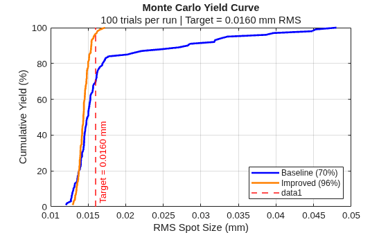
The baseline curve shows the initial yield from the fabrication experience. If the baseline yield is already acceptable, no further improvement is required. The improved curve shows the yield after tightening the top 5 offenders identified by the sensitivity analysis and widening the compensator range. Observe that after improvement, the distribution shifts leftward toward smaller spot sizes. Initially, only 70% of the trials had a spot size less than the target spot size of 0.016 mm, whereas after improvement this proportion increased to 96%.

If yield is still not acceptable after one iteration of improvement, repeat the process. Run sensitivity analysis on the new tolerance set and get the new ranking, tighten the new worst offenders, and rerun the Monte Carlo tolerancing analysis to compute the new yield.

Supporting Functions

buildParameterLabels

This function builds readable display labels for each tolerance parameter.

function labels = buildParameterLabels(paramNames,paramTypes,targetIndices)
    numTol = numel(paramNames);
    labels = strings(numTol,1);
    for numTol = 1:numTol
        if paramNames(numTol)== "Radius"
            labels(numTol) = "Radius (Surface " + string(targetIndices(numTol)) + ")";
        elseif contains(paramTypes(numTol),"SurfacePosition")
            labels(numTol) = "Thickness (Surface " + string(targetIndices(numTol)) + ")";
        elseif contains(paramTypes(numTol),"ComponentPosition")
            labels(numTol) = "Air Gap (Component " + string(targetIndices(numTol)) + ")";
        elseif paramNames(numTol)=="Nd"
            labels(numTol) = "Refractive Index (Component " + string(targetIndices(numTol)) + ")";
        elseif paramNames(numTol)=="Vd"
            labels(numTol) = "Abbe Number (Component " + string(targetIndices(numTol)) + ")";
        end
    end
end

buildTightenedToleranceSet

This function builds a new tolerance set with specified parameters tightened by a given factor. This function uses the getInitialTolerance supporting function, which is defined later in this section.

function tightenedTolSet = buildTightenedToleranceSet(~,tbl,tightenIdx,factor)
    paramNames = tbl.TargetProperty;
    paramTypes = tbl.TargetPropertyType;
    targetIndices = tbl.TargetIndex;
    numTol = height(tbl);
    
    tightenedTolSet = opticalToleranceSet;
    for idx = 1:numTol
        ft = getInitialTolerance(paramNames(idx),paramTypes(idx));
    
        % Tighten if this parameter is in the tighten list
        if ismember(idx,tightenIdx)
            ft = ft*factor;
        end
    
        tolRange = [-ft ft];
        if paramNames(idx)=="Radius"
            tightenedTolSet = addSurfaceRadiusTolerance(tightenedTolSet,tolRange, ...
                TargetIndex=targetIndices(idx));
        elseif contains(paramTypes(idx),"SurfacePosition")
            tightenedTolSet = addSurfacePositionTolerance(tightenedTolSet,PositionZ=tolRange, ...
                TargetIndex=targetIndices(idx));
        elseif contains(paramTypes(idx),"ComponentPosition")
            tightenedTolSet = addComponentPositionTolerance(tightenedTolSet,PositionZ=tolRange, ...
                TargetIndex=targetIndices(idx));
        elseif paramNames(idx)=="Nd"
            tightenedTolSet = addComponentMaterialTolerance(tightenedTolSet,Nd=tolRange, ...
                TargetIndex=targetIndices(idx));
        elseif paramNames(idx)=="Vd"
            tightenedTolSet = addComponentMaterialTolerance(tightenedTolSet,Vd=tolRange, ...
                TargetIndex=targetIndices(idx));
        end
    end
end

getTolValues

This function extracts the initial tolerance half-range values for specified parameter indices, based on their type. This function uses the getInitialTolerance supporting function, which is defined later in this section.

function tolValues = getTolValues(tbl,indices)
    tolValues = zeros(numel(indices),1);
    for idx = 1:numel(indices)
        tolValues(idx) = getInitialTolerance(tbl.TargetProperty(indices(idx)),tbl.TargetPropertyType(indices(idx)));
    end
end

getInitialTolerance

This function returns the initial tolerance half-range for a parameter, based on its type.

function ft = getInitialTolerance(paramName,paramType)
    if paramName=="Radius"
        ft = 0.1;
    elseif contains(paramType,"SurfacePosition")
        ft = 0.05;
    elseif contains(paramType,"ComponentPosition")
        ft = 0.08;
    elseif paramName=="Nd"
        ft = 0.0005;
    elseif paramName=="Vd"
        ft = 0.5;
    else
        ft = 0;
    end
end