Troubleshoot Frequency-Domain Identification of Transfer Function Models
This example shows how to perform and troubleshoot the identification of a SISO system using frequency-response data (FRD). The techniques explained here can also be applied to MIMO models and frequency-domain input-output data.
When you use the tfest command to estimate a SISO transfer function model from the frequency-response data, the estimation algorithm minimizes the following least-squares loss (cost) function:
Here W is a frequency-dependent weight that you specify, G is the transfer function that is to be estimated, f is the measured frequency-response data, and is the frequency. Nf is the number frequencies at which the data is available. is the frequency-response error.
In this example, you first estimate the model without preprocessing the data or using estimation options to specify a weighting filter. You then apply these troubleshooting techniques to improve the model estimation.
Estimate the Model Without Preprocessing and Filtering
Load the measured continuous-time frequency response data.
load troubleshooting_example_data Gfrd;
Gfrd is an idfrd object that stores the data.
Estimate an initial transfer function model with 11 poles and 10 zeros by using the estimation data.
Gfit = tfest(Gfrd,11,10);
Plot the frequency-response magnitude of the estimated model and the measured frequency-response data.
bodemag(Gfrd,Gfit);
ylim([-100 0])
legend('Measured','Estimated')

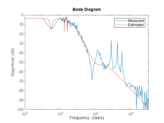
The estimated model contains spurious dynamics. The estimation algorithm misses the valley at 60 rad/s and the resonant peaks after that. Therefore, the model is not a good fit to the data.
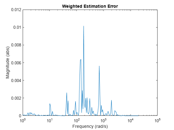
The algorithm minimizes the squared error magnitude, , in the loss function. Plot this quantity as a function of frequency. This error plot provides a view of which data points contribute the most to the loss function, and so are the likely limiting factors during estimation. The plot can help you identify why there are spurious or uncaptured dynamics.
Because you have not specified a frequency-dependent weight, is 1.
w = Gfrd.Frequency;
r1 = squeeze(freqresp(Gfit,w));
r2 = squeeze(freqresp(Gfrd,w));
fitError = r1-r2;
semilogx(w,abs(fitError).^2)
title('Weighted Estimation Error');
xlabel('Frequency (rad/s)');
ylabel('Magnitude (abs)')

From the data, model, and error plots you can see that:
The largest fitting errors are below 10 rad/s.
The algorithm focusses on fitting the noisy high magnitude data points below 10 rad/s, which have a large contribution to the optimization loss function. As a result, the algorithm assigns spurious poles and zeros to this data region. To address this issue, you can preprocess the data to improve signal-to-noise ratio in this region. You can also use frequency-dependent weights to make the algorithm put less focus on this region.
Below approximately 40 rad/s, most variations in data are due to noise. There are no significant system modes (valleys or peaks) in the data. To address this issue, you can use a moving-average filter over the data to smooth the measured response.
The algorithm ignores the valley around 60 rad/s and the three lightly damped resonant peaks that follow it. These features contribute little to the loss function because the fitting error is small at these frequencies. To address this issue, you can specify frequency-dependent weights to make the algorithm pay more attention to these frequencies.
Preprocess Data
To improve the estimated model quality, preprocess the data. To do so, you truncate the low signal-to-noise portions of data below 1 rad/s and above 2e4 rad/s that are not interesting. Then you use a moving-average filter to smooth data in the low-frequency high-magnitude region below 40 rad/s. At these frequencies, the data has a low signal-to-noise ratio, but has dynamics that you are interested in capturing. Do not apply the filter at frequencies above 40 rad/s to avoid smoothing data where you see the valley and the three peaks that follow it.
Make a copy of the original idfrd data object.
GfrdProcessed = Gfrd;
Truncate the data below 1 rad/s and above 2e4 rad/s.
GfrdProcessed = fselect(GfrdProcessed,1,2e4);
Apply a three-point centered moving-average filter to smooth out the frequency-response data below 40 rad/s that contains spurious dynamics. The response data is stored in the ResponseData property of the object.
w = GfrdProcessed.Frequency;
f = squeeze(GfrdProcessed.ResponseData);
idx = w<40;
f(idx) = movmean(f(idx),3);
Here f(idx) is the frequency-response data at frequencies less than 40 rad/s.
Place the filtered data back into the original data object.
GfrdProcessed.ResponseData = f;
Plot the original and preprocessed data.
bodemag(Gfrd,GfrdProcessed);
ylim([-100 0]);
legend('Original data','Preprocessed data');

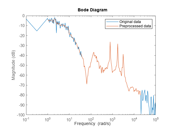
The plot shows that all desired dynamics are intact after preprocessing.
Specify Weighting Filter
Use a low weight for the low frequency region under 10 rad/s where spurious dynamics exist. This low weight and the smoothing applied earlier to this data reduce the chance of spurious peaks in the estimated model response in this region.
Weight = ones(size(f));
idx = w<10;
Weight(idx) = Weight(idx)/10;
Use a high weight for data in the frequency range 40-6e3 rad/s where you want to capture the dynamics but the response data magnitude is low.
idx = w>40 & w<6e3;
Weight(idx) = Weight(idx)*30;
Specify the weights in the WeightingFilter option of the estimation option set.
tfestOpt = tfestOptions('WeightingFilter',Weight);Note that Weight is a custom weighting filter. You can also specify WeightingFilter as 'inv' or 'invsqrt' for frequency-response data. These options specify the weight as and , respectively. These options enable you to quickly test the effect of using a higher weight for low magnitude regions of data. 'invsqrt' is typically a good initial choice. If these weights do not yield good estimation results, you can provide custom weights as shown in this example.
Estimate Model Using Preprocessed and Filtered Data
Estimate a transfer function model with 11 poles and 10 zeros using the preprocessed data and specified weighting filter.
GfitNew = tfest(GfrdProcessed,11,10,tfestOpt);
Plot the original data, the initial model response, and the new model response.
bodemag(Gfrd,Gfit,GfitNew);
ylim([-100 0]);
legend('Original Data','Original Model','New Model');

Plot the estimation error. Compute the estimation error by including the weighting filter Weight that you used for estimating GfitNew.
w = GfrdProcessed.Frequency;
r1 = squeeze(freqresp(GfitNew,w));
r2 = squeeze(freqresp(GfrdProcessed,w));
fitErrorNew = Weight.*(r1-r2);
semilogx(w,abs(fitErrorNew).^2)
title('Weighted Estimation Error');
xlabel('Frequency (rad/s)');
ylabel('Magnitude (abs)');

The new model successfully captures all system dynamics of interest.
You can use the weighted error plot for further troubleshooting if your initial choice of weights does not yield a satisfactory result.