segment
Segment data and estimate models for each segment
Syntax
segm = segment(z,nn)
[segm,V,thm,R2e] = segment(z,nn,R2,q,R1,M,th0,P0,ll,mu)
Description
segment builds models of AR, ARX, or ARMAX/ARMA
type,
assuming that the model parameters are piecewise constant over time. It results in a model that has split the data record into segments over which the model remains constant. The function models signals and systems that might undergo abrupt changes.
The input-output data is contained in z,
which is either an iddata object or a matrix z
= [y u] where y and u are
column vectors. If the system has several inputs, u has
the corresponding number of columns.
The argument nn defines the model order.
For the ARMAX model
nn = [na nb nc nk];
where na, nb, and nc are
the orders of the corresponding polynomials. See What Are Polynomial Models?. Moreover, nk is
the delay. If the model has several inputs, nb and nk are
row vectors, giving the orders and delays for each input.
For an ARX model (nc = 0) enter
nn = [na nb nk];
For an ARMA model of a time series
z = y;
nn = [na nc];
and for an AR model
nn = na;
The output argument segm is a matrix, where
the kth row contains the parameters corresponding
to time k. This is analogous to output estimates
returned by the recursiveARX and recursiveARMAX estimators. The output
argument thm of segment contains
the corresponding model parameters that have not yet been segmented.
Each row of thm contains the parameter estimates
at the corresponding time instant. These estimates are formed by weighting
together the parameters of M (default:
5) different time-varying models, with the participating models changing
at every time step. Consider segment as
an alternative to the online estimation commands when you are not
interested in continuously tracking the changes in parameters of a
single model, but need to detect abrupt changes in the system dynamics.
The output argument V contains the sum of
the squared prediction errors of the segmented model. It is a measure
of how successful the segmentation has been.
The input argument R2 is the assumed variance
of the innovations e(t)
in the model. The default value of R2, R2
= [], is that it is estimated. Then the output argument R2e is
a vector whose kth element contains the estimate
of R2 at time k.
The argument q is the probability that the
model exhibits an abrupt change at any given time. The default value
is 0.01.
R1 is the assumed covariance matrix of the
parameter jumps when they occur. The default value is the identity
matrix with dimension equal to the number of estimated parameters.
M is the number of parallel models used in
the algorithm (see below). Its default value is 5.
th0 is the initial value of the parameters.
Its default is zero. P0 is the initial covariance
matrix of the parameters. The default is 10 times the identity matrix.
ll is the guaranteed life of each of the
models. That is, any created candidate model is not abolished until
after at least ll time steps. The default is ll
= 1. Mu is a forgetting parameter that
is used in the scheme that estimates R2. The default
is 0.97.
The most critical parameter for you to choose is R2.
It is usually more robust to have a reasonable guess of R2 than
to estimate it. Typically, you need to try different values of R2 and
evaluate the results. (See the example below.) sqrt(R2) corresponds
to a change in the value y(t)
that is normal, giving no indication that the system or the input
might have changed.
Examples
Create a sinusoid for the simulated model output.
y = sin([1:50]/3)';
Specify the input signal to be constant at 1.
u = ones(size(y));
Specify the estimated noise variance for the model.
R2 = 0.1;
Segment the signal and estimate an ARX model for each segment. Use the simple model , where is the model parameter describing the piecewise constant level of the estimated output, .
segm = segment([y,u],[0 1 1],R2);
Examine the result.
plot([segm,y])
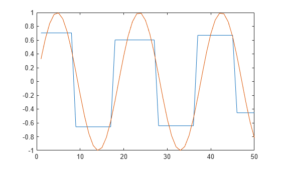
Vary the value of R2 to change the estimated noise variance. Decreasing R2 increases the number of segments produced for this model.
Load and plot the estimation data.
load iddemo6m.mat z
z = iddata(z(:,1),z(:,2));
plot(z)
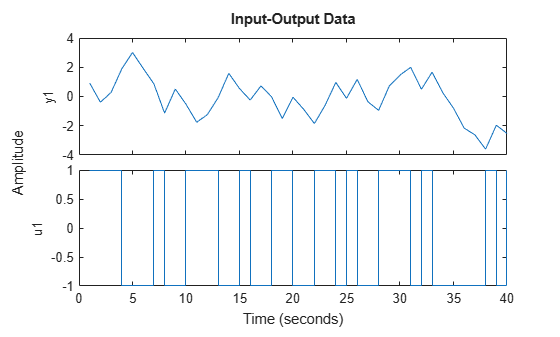
This data contains a change in time delay from 2 to 1, which is difficult to detect by examining the data.
Specify the model orders to estimate an ARX model of the form:
nn = [1 2 1];
Segment the data and estimate ARX models for each segment. Specify an estimated noise variance of 0.1.
seg = segment(z,nn,0.1);
Examine the parameters of the segmented model.
plot(seg)
legend('a','b1','b2');
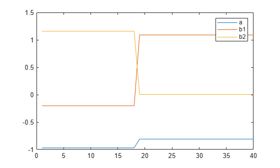
The data has been divided into two segments, as indicated by the change in model parameters around sample number 19. The increase in b1, along with a corresponding decrease in b2, shows the change in model delay.
Limitations
segment is not compatible with MATLAB®
Coder™ or MATLAB
Compiler™.
Algorithms
The algorithm is based on M parallel models,
each recursively estimated by an algorithm of Kalman filter type.
Each model is updated independently, and its posterior probability
is computed. The time-varying estimate thm is formed
by weighting together the M different models with
weights equal to their posterior probability. At each time step the
model (among those that have lived at least ll samples)
that has the lowest posterior probability is abolished. A new model
is started, assuming that the system parameters have changed, with
probability q, a random jump from the most likely
among the models. The covariance matrix of the parameter change is
set to R1.
After all the data are examined, the surviving model with the
highest posterior probability is tracked back and the time instances
where it jumped are marked. This defines the different segments of
the data. (If no models had been abolished in the algorithm, this
would have been the maximum likelihood estimates of the jump instances.)
The segmented model segm is then formed by smoothing
the parameter estimate, assuming that the jump instances are correct.
In other words, the last estimate over a segment is chosen to represent
the whole segment.
Version History
Introduced before R2006a