Compare paretosearch and gamultiobj
R2026bThis example shows how to create a set of points on the Pareto front using both paretosearch and gamultiobj. The objective function mymulti3 has two objectives and a two-dimensional control variable x. For speed of calculation, the function is vectorized.
function f = mymulti3(x)
%
f(:,1) = x(:,1).^4 + x(:,2).^4 + x(:,1).*x(:,2) - (x(:,1).^2).*(x(:,2).^2) - 9*x(:,1).^2;
f(:,2) = x(:,2).^4 + x(:,1).^4 + x(:,1).*x(:,2) - (x(:,1).^2).*(x(:,2).^2) + 3*x(:,2).^3;
end
Basic Example and Plots
Find Pareto sets for the objective functions using paretosearch and gamultiobj. Set the UseVectorized option to true for added speed. Include a plot function to visualize the Pareto set.
rng default
nvars = 2;
opts = optimoptions(@gamultiobj,UseVectorized=true,PlotFcn="gaplotpareto");
[xga,fvalga,~,gaoutput] = gamultiobj(@(x)mymulti3(x),nvars,[],[],[],[],[],[],[],opts);
gamultiobj stopped because the average change in the spread of Pareto solutions is less than options.FunctionTolerance.
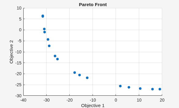
optsp = optimoptions("paretosearch",UseVectorized=true,PlotFcn=["psplotparetof" "psplotparetox"]);
[xp,fvalp,~,psoutput] = paretosearch(@(x)mymulti3(x),nvars,[],[],[],[],[],[],[],optsp);
Pareto set found that satisfies the constraints.

Optimization completed because the relative change in the volume of the Pareto set
is less than 'options.ParetoSetChangeTolerance' and constraints are satisfied to within
'options.ConstraintTolerance'.
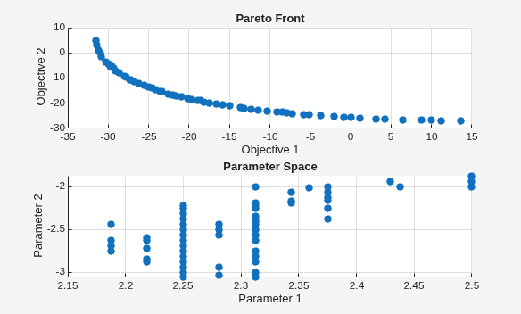
Compute theoretically exact points on the Pareto front by using mymulti4.
function mout = mymulti4(x)
%
gg = [4*x(1)^3+x(2)-2*x(1)*(x(2)^2) - 18*x(1);
    x(1)+4*x(2)^3-2*(x(1)^2)*x(2)];
gf = gg + [18*x(1);9*x(2)^2];

mout = gf(1)*gg(2) - gf(2)*gg(1);
end
The mymulti4 function evaluates the gradients of the two objective functions. Next, for a range of values of x(2), use fzero to locate the point where the gradients are exactly parallel, which is where the output mout = 0.
a = [fzero(@(t)mymulti4([t,-3.15]),[2,3]),-3.15];
for jj = linspace(-3.125,-1.89,50)
    a = [a;[fzero(@(t)mymulti4([t,jj]),[2,3]),jj]];
end
figure
plot(fvalp(:,1),fvalp(:,2),"bo");
hold on
fs = mymulti3(a);
plot(fvalga(:,1),fvalga(:,2),"r*");
plot(fs(:,1),fs(:,2),"k.")
legend("Paretosearch","Gamultiobj","True")
xlabel("Objective 1")
ylabel("Objective 2")
hold off
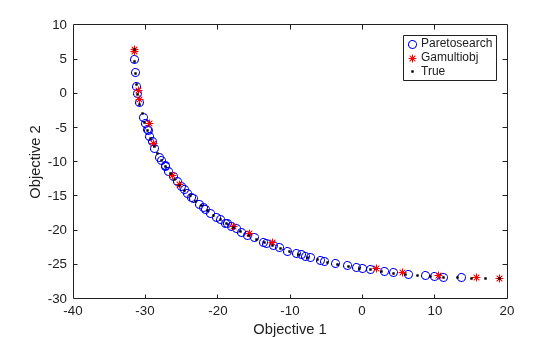
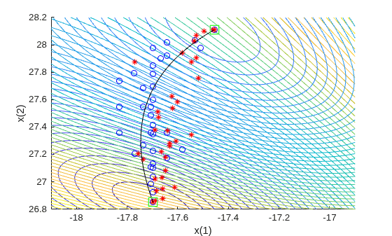
gamultiobj finds points with a slightly wider spread in objective function space. Plot the solutions in decision variable space, along with the theoretical optimal Pareto curve and a contour plot of the two objective functions.
[x,y] = meshgrid(1.9:.01:3.1,-3.2:.01:-1.8);
mydata = mymulti3([x(:),y(:)]);
myff = sqrt(mydata(:,1) + 39);% Spaces the contours better
mygg = sqrt(mydata(:,2) + 28);% Spaces the contours better
myff = reshape(myff,size(x));
mygg = reshape(mygg,size(x));

figure;
hold on
contour(x,y,mygg,50)
contour(x,y,myff,50)
plot(xp(:,1),xp(:,2),"bo")
plot(xga(:,1),xga(:,2),"r*")
plot(a(:,1),a(:,2),"-k")
xlabel("x(1)")
ylabel("x(2)")
hold off
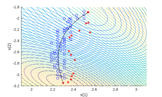
Unlike the paretosearch solution, the gamultiobj solution has points at the extreme ends of the range in objective function space. However, the paretosearch solution has more points that are closer to the true solution in both objective function space and decision variable space. The number of points on the Pareto front is different for each solver when you use the default options.
Shifted Problem
What happens if the solution to your problem has control variables that are large? Examine this case by shifting the problem variables. For an unconstrained problem, gamultiobj can fail, while paretosearch is more robust to such shifts.
For easier comparison, specify 35 points on the Pareto front for each solver.
shift = [20,-30];
fun = @(x)mymulti3(x+shift);
opts.PopulationSize = 100; % opts.ParetoFraction = 35
[xgash,fvalgash,~,gashoutput] = gamultiobj(fun,nvars,[],[],[],[],[],[],opts);
gamultiobj stopped because the average change in the spread of Pareto solutions is less than options.FunctionTolerance.
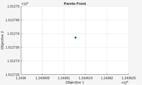
gamultiobj fails to find a useful Pareto set.
optsp.PlotFcn = [];
optsp.ParetoSetSize = 35;
[xpsh,fvalpsh,~,pshoutput] = paretosearch(fun,nvars,[],[],[],[],[],[],[],optsp);
Pareto set found that satisfies the constraints.

Optimization completed because the relative change in the volume of the Pareto set
is less than 'options.ParetoSetChangeTolerance' and constraints are satisfied to within
'options.ConstraintTolerance'.
figure
plot(fvalpsh(:,1),fvalpsh(:,2),"bo");
hold on
plot(fs(:,1),fs(:,2),"k.")
legend("Paretosearch","True")
xlabel("Objective 1")
ylabel("Objective 2")
hold off
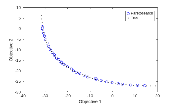
paretosearch finds solution points spread evenly over nearly the entire possible range.
Adding bounds, even fairly loose ones, helps both gamultiobj and paretosearch to find appropriate solutions. Set lower bounds of -50 in each component, and upper bounds of 50.
opts.PlotFcn = [];
optsp.PlotFcn = [];
lb = [-50,-50];
ub = -lb;
[xgash,fvalgash,~,gashoutput] = gamultiobj(fun,nvars,[],[],[],[],lb,ub,opts);
gamultiobj stopped because the average change in the spread of Pareto solutions is less than options.FunctionTolerance.
[xpsh2,fvalpsh2,~,pshoutput2] = paretosearch(fun,nvars,[],[],[],[],lb,ub,[],optsp);
Pareto set found that satisfies the constraints.

Optimization completed because the relative change in the volume of the Pareto set
is less than 'options.ParetoSetChangeTolerance' and constraints are satisfied to within
'options.ConstraintTolerance'.
figure
plot(fvalpsh2(:,1),fvalpsh2(:,2),"bo");
hold on
plot(fvalgash(:,1),fvalgash(:,2),"r*");
plot(fs(:,1),fs(:,2),"k.")
legend("Paretosearch","Gamultiobj","True")
xlabel("Objective 1")
ylabel("Objective 2")
hold off
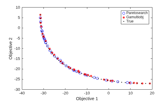
In this case, both solvers find good solutions.
Start paretosearch from gamultiobj Solution
Obtain a similar range of solutions from the solvers by starting paretosearch from the gamultiobj solution.
optsp.InitialPoints = xgash;
[xpsh3,fvalpsh3,~,pshoutput3] = paretosearch(fun,nvars,[],[],[],[],lb,ub,[],optsp);
Pareto set found that satisfies the constraints.

Optimization completed because the relative change in the volume of the Pareto set
is less than 'options.ParetoSetChangeTolerance' and constraints are satisfied to within
'options.ConstraintTolerance'.
figure
plot(fvalpsh3(:,1),fvalpsh3(:,2),"bo");
hold on
plot(fvalgash(:,1),fvalgash(:,2),"r*");
plot(fs(:,1),fs(:,2),"k.")
legend("Paretosearch","Gamultiobj","True")
xlabel("Objective 1")
ylabel("Objective 2")
hold off
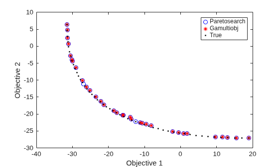
Now the paretosearch solution is similar to the gamultiobj solution, although some of the solution points differ.
Start from Single-Objective Solutions
Another way of obtaining a good solution is to start from the points that minimize each objective function separately.
From the multiobjective function, create a single-objective function that chooses each objective in turn. Use the shifted function from the previous section. Because you are giving good start points to the solvers, you do not need to specify bounds.
nobj = 2; % Number of objectives

x0 = -shift; % Initial point for single-objective minimization
uncmin = cell(nobj,1); % Cell array to hold the single-objective minima
allfuns = zeros(nobj,2); % Hold the objective function values
eflag = zeros(nobj,1);
fopts = optimoptions("patternsearch",Display="off"); % Use an appropriate solver here
for i = 1:nobj
    indi = zeros(nobj,1); % Choose the objective to minimize
    indi(i) = 1;
    funi = @(x)dot(fun(x),indi);
    [uncmin{i},~,eflag(i)] = patternsearch(funi,x0,[],[],[],[],[],[],[],fopts); % Minimize objective i
    allfuns(i,:) = fun(uncmin{i});
end
uncmin = cell2mat(uncmin); % Matrix of start points
Start paretosearch from the single-objective minimum points and note that it has a full range in its solutions. paretosearch adds random initial points to the supplied ones in order to have a population of at least options.ParetoSetSize individuals. Similarly, gamultiobj adds random points to the supplied ones to obtain a population of at least (options.PopulationSize)*(options.ParetoFraction) individuals.
optsp = optimoptions(optsp,InitialPoints=uncmin);
[xpinit,fvalpinit,~,outputpinit] = paretosearch(fun,nvars,[],[],[],[],[],[],[],optsp);
Pareto set found that satisfies the constraints.

Optimization completed because the relative change in the volume of the Pareto set
is less than 'options.ParetoSetChangeTolerance' and constraints are satisfied to within
'options.ConstraintTolerance'.
Now solve the problem using gamultiobj starting from the initial points.
opts = optimoptions(opts,InitialPopulationMatrix=uncmin);
[xgash2,fvalgash2,~,gashoutput2] = gamultiobj(fun,nvars,[],[],[],[],[],[],opts);
gamultiobj stopped because the average change in the spread of Pareto solutions is less than options.FunctionTolerance.
figure
plot(fvalpinit(:,1),fvalpinit(:,2),"bo");
hold on
plot(fvalgash2(:,1),fvalgash2(:,2),"r*");
plot(fs(:,1),fs(:,2),"k.")
plot(allfuns(:,1),allfuns(:,2),"gs",MarkerSize=12)
legend("Paretosearch","Gamultiobj","True","Start Points")
xlabel("Objective 1")
ylabel("Objective 2")
hold off
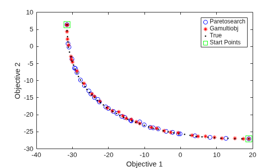
Both solvers fill in the Pareto front between the extreme points, with reasonably accurate and well-spaced solutions.
View the final points in decision variable space.
figure;
hold on
xx = x - shift(1);
yy = y - shift(2);
contour(xx,yy,mygg,50)
contour(xx,yy,myff,50)
plot(xpinit(:,1),xpinit(:,2),"bo")
plot(xgash2(:,1),xgash2(:,2),"r*")
ashift = a - shift;
plot(ashift(:,1),ashift(:,2),"-k")
plot(uncmin(:,1),uncmin(:,2),"gs",MarkerSize=12);
xlabel("x(1)")
ylabel("x(2)")
hold off