Design Fusion Filter for Custom Sensors
This example introduces how to customize sensor models used with an insEKF object.
Using the insEKF object, you can fuse measurement data from multiple types of sensors by using the built-in INS sensor models, including the insAccelerometer, insGyrospace, insMagnetomer, and insGPS objects. Though these sensor objects cover a variety of INS sensor models, you may want to fuse measurement data from a different type of sensor. Using the insEKF object through an extended framework, you can define your own sensor models and motion models used by the filter. In this example, you learn how to customize three sensor models in a few steps. You can apply the similar steps for defining a motion model.
This example requires the Sensor Fusion and Tracking Toolbox™ or the Navigation Toolbox™. This example also optionally uses MATLAB® Coder™ to accelerate filter tuning.
Problem Description
Consider you are trying to estimate the position of an object that moves in one dimension. To estimate the position, you use a velocity sensor and fuse data from that sensor to determine the position. Typically, applying this approach can lead to a poor estimate of position because small errors in the velocity estimate can integrate to form larger errors in the position estimate. As shown later in this example, combining measurements from multiple sensors can improve the results.
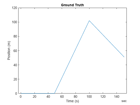
To start, define a simple ground truth trajectory for the object and visualize how it moves.
groundTruth = exampleHelperMakeGroundTruth();
plot(groundTruth.Time, groundTruth.Position);
xlabel("Time (s)");
ylabel("Position (m)");
title("Ground Truth");
snapnow;
Simple Velocity Sensor
Consider the data from a simple velocity sensor that measures velocity but is corrupted by a small bias and additive white Gaussian noise.
velBias = exampleHelperVelocityWithBias(groundTruth);
For the simplest approach, you create a filter that treats the velocity measurements as just velocity plus white noise. This will likely not produce desirable results, but it is worth trying the simplest model first. To create a velocity sensor model for the insEKF object, you need to define a class that inherits from the positioning.INSSensorModel interface class. At minimum you need to implement a measurement method which takes the sensor object and filter object as inputs. The measurement method returns a vector z as an estimate of measurement from the sensor, based on state variables.
classdef exampleHelperVelocitySensor < positioning.INSSensorModel
%EXAMPLEHELPERVELOCITYSENSOR A simple velocity sensor for insEKF
% This class is for internal use only. It may be removed in the future.

%   Copyright 2021 The MathWorks, Inc.

    methods
        function z = measurement(~, filt)
            % The measurement is just the velocity estimate
            z = stateparts(filt, 'Velocity');
        end
    end
end
This is the minimum required to define a sensor that works with the insEKF object. You could optionally define the measurement Jacobian in the measurementJacobian method, which can improve the calculation speed and possibly improve the estimation accuracy. Without implementing the measurementJacobian method, you are relying on the insEKF to numerically compute the Jacobian.
You build the filter with a simple 1-D constant velocity motion model defined using a BasicConstantVelocityMotion class. This class is an example of how to implement your own custom motion models by inheriting from the positioning.INSMotionModel interface class. Defining custom motion models requires implementing only a subset of the methods required to implement a custom sensor model.
You can now build the filter, tune its noise parameters, and see how it performs. You can name the Velocity sensor "VelocityWithBias" using the insOptions object.
basicOpts = insOptions(SensorNamesSource="property", SensorNames={'VelocityWithBias'});
basicfilt = insEKF(exampleHelperVelocitySensor, exampleHelperConstantVelocityMotion, ...
    basicOpts);
The object starts at rest with a position of zero. Set the state covariance for the position and velocity to a lower value before tuning.
statecovparts(basicfilt, "Position", 1e-2);
statecovparts(basicfilt, "Velocity", 1e-2);
Tune the filter after specifying a noise structure and a tunerconfig object.
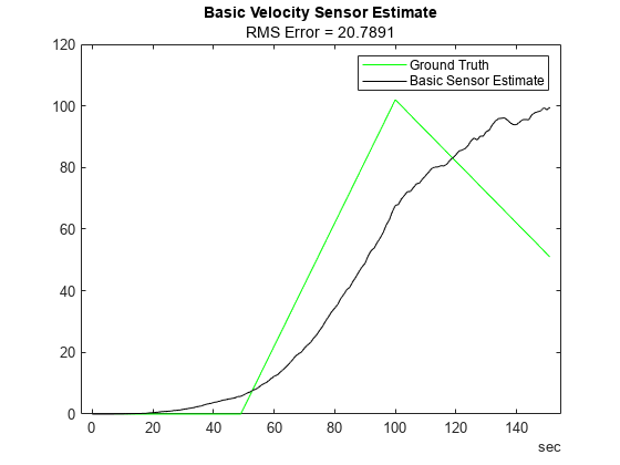
mn = tunernoise(basicfilt);
tunerIters = 30;
cfg = tunerconfig(basicfilt, MaxIterations=tunerIters, Display='none');
tunedmn = tune(basicfilt, mn, velBias, groundTruth, cfg);

estBasic = estimateStates(basicfilt, velBias, tunedmn);
figure;
plot(groundTruth.Time, groundTruth.Position, 'g', estBasic.Time, ...
    estBasic.Position, 'k')
title("Basic Velocity Sensor Estimate");
err = sqrt(mean((estBasic.Position - groundTruth.Position).^2));
subtitle("RMS Error = " + err);
legend("Ground Truth", "Basic Sensor Estimate");
snapnow;
The estimation results are poor as expected since the bias is not accounted for by the filter. When the unaccounted velocity bias is integrated into position, the estimate diverges quickly from ground truth.
Velocity Sensor with Bias
Now you can explore a more complex sensor model which accounts for the sensor bias. To do this, you define a sensorstates method to inform the insEKF to track the sensor bias in its state vector, saved in the State property of the filter. You can query the sensor bias with the stateparts object function of the filter and use the bias estimate in the measurement function.
classdef exampleHelperVelocitySensorWithBias < positioning.INSSensorModel
%EXAMPLEHELPERVELOCITYSENSORWITHBIAS Velocity sensor assuming constant bias
% This class is for internal use only. It may be removed in the future.

%   Copyright 2021 The MathWorks, Inc.

    methods
        function s = sensorstates(~,~)
            % Assume there is a constant bias corrupting the velocity
            % measurement. Estimate that bias as part of the filter
            % computation.
            s = struct('Bias', 0);
        end
        function z = measurement(sensor, filt)
            % Measurement is velocity plus bias. Obtain the velocity from
            % the filter state.
            velocity = stateparts(filt, 'Velocity');

            % Obtain the sensor bias from the filter state by directly
            % using the sensor object as an input to the stateparts object
            % function. In this way, knowledge of the SensorName associated
            % with this sensor is not required. See the reference page for
            % stateparts for more details.
            bias = stateparts(filt, sensor, 'Bias');

            % Form the measurement
            z = velocity + bias;
        end
        function dzdx = measurementJacobian(sensor, filt)
            % Compute the Jacobian as the partial derivates of the Bias
            % state relative to all other states.
            N = numel(filt.State);  % Number of states

            % Initialize a matrix of partial derivatives. This matrix has
            % one row because the sensor state is a scalar.
            dzdx = zeros(1,N);

            % The partial derivative of z with respect to the Bias is 1. So
            % put a 1 at the Bias index in the dzdx matrix:
            bidx = stateinfo(filt, sensor, 'Bias');
            dzdx(:,bidx) = 1;

            % The partial derivative of z with respect to the Velocity is
            % also 1. So put a 1 at the Bias index in the dzdx matrix:
            vidx = stateinfo(filt, 'Velocity');
            dzdx(:,vidx) = 1;
        end
    end

end
In the above you implemented the measurementJacobian method rather than relying on a numeric Jacobian. The Jacobian matrix contains the partial derivatives of the sensor measurement with respect to the filter state, which is an M-by-N matrix, where M is the number of elements in the vector returned by the measurement method and N is the number of states of the filter. Now you can build a filter with the custom sensor.
sensorVelWithBias = exampleHelperVelocitySensorWithBias;
velWithBiasFilt = insEKF(sensorVelWithBias, ...
    exampleHelperConstantVelocityMotion, basicOpts);
You can set the initial bias state of the filter with an estimate of the bias, based on data collected while the sensor is stationary, using the stateparts object function.
stationaryLen = 1e7;
stationary = timetable(zeros(stationaryLen,1), zeros(stationaryLen,1), ...
    TimeStep=groundTruth.Properties.TimeStep, ...
    VariableNames={'Position', 'Velocity'});
biasCalibrationData = exampleHelperVelocityWithBias(stationary);

stateparts(velWithBiasFilt,  sensorVelWithBias, "Bias", ...
    mean(biasCalibrationData.VelocityWithBias));
Again, set the state covariance for these states to smaller values before tuning.
statecovparts(velWithBiasFilt, "Position", 1e-2);
statecovparts(velWithBiasFilt, "Velocity", 1e-2);
You can tune this filter as previously, but you can also tune it faster using MATLAB Coder. While the tune object function does not support code generation, you can use a MEX-accelerated cost function to greatly increase the tuning speed. You can specify the tune function to use a custom cost function through the tunerconfig input. The insEKF object has object functions to help create a custom cost function. The createTunerCostTemplate object function creates a cost function, which tries to minimize the RMS error of state estimates, in a new document in the Editor. You can then generate code for that function with the help of the tunerCostFcnParam object function, which creates an example of the first argument to a cost function.
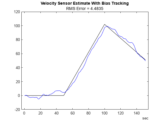
% Use MATLAB Coder to accelerate tuning by MEXing the cost function.
% To run the MATLAB Coder accelerated path, prior to running the example,
% type:
%   exampleHelperUseCodegenForCost(true);
% To avoid using MATLAB Coder, prior to the example, type:
%   exampleHelperUseCodegenForCost(false);

useCodegenForTuning = exampleHelperUseCodegenForCost();

if useCodegenForTuning
    createTunerCostTemplate(velWithBiasFilt); % A new cost function in the editor
    exampleHelperSaveCostFunction;
    p = tunerCostFcnParam(velWithBiasFilt);
    % Now generate a mex file
    codegen tunercost.m -args {p, velBias, groundTruth};
    % Use the Custom Cost Function
    cfg2 = tunerconfig(velWithBiasFilt, MaxIterations=tunerIters, ...
        Cost="custom", CustomCostFcn=@tunercost_mex, Display='none');
else
    % Use the default cost function
    cfg2 = tunerconfig(velWithBiasFilt, MaxIterations=tunerIters, ...
        Display='none'); %#ok<*UNRCH>
end
mn = tunernoise(velWithBiasFilt);
tunedmn = tune(velWithBiasFilt, mn, velBias, groundTruth, cfg2);
estWithBias = estimateStates(velWithBiasFilt, velBias, tunedmn);
figure;
plot(groundTruth.Time, groundTruth.Position, 'k', estWithBias.Time, ...
    estWithBias.Position, 'b')
title("Velocity Sensor Estimate With Bias Tracking");
err = sqrt(mean((estWithBias.Position - groundTruth.Position).^2));
subtitle("RMS Error = " + err);
snapnow;
From the results, the position estimate has improved but is still not ideal. The filter estimates the bias, but any error in the bias estimate is treated as real velocity, which corrupts the position estimate. A more sophisticated sensor model can further improve the results.
Velocity Sensor with Gauss-Markov Noise
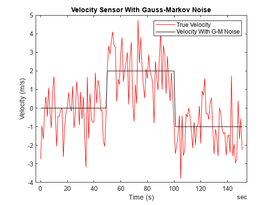
Consider a new velocity sensor model that is corrupted with first-order Gauss-Markov noise.
velGM = exampleHelperVelocityWithGaussMarkov(groundTruth);
figure
plot(velGM.Time, velGM.VelocityWithGM, 'r', groundTruth.Time, ...
    groundTruth.Velocity, 'k');
title("Velocity Sensor With Gauss-Markov Noise");
xlabel("Time (s)");
ylabel("Velocity (m/s)");
legend("True Velocity", "Velocity With G-M Noise");
snapnow;
First-order Gauss-Markov noise can be modeled in discrete time as:
where is white noise. The equivalent continuous time formulation is:
where is the time constant of the process, and w(t) and x(t) are the continuous time versions of the discrete state and process noise , respectively.
You can check that these are a valid discrete-continuous pair by applying Euler integration on the second equation between time k and k-1 to obtain the first equation. See Reference [1] for a further explanation. For simplicity, set as 0.002 for this example. Since the Gauss-Markov process evolves over time you need to implement it in the stateTransition method of the positioning.INSSensorModel class. The stateTransition method describes how state elements described in sensorstates evolve over time. The stateTransition function outputs a structure with the same fields as the output structure of the sensorstates method, and each field contains the derivative of the state with respect to time. When the stateTransition method is not implemented explicitly, the insEKF object assumes the state is constant over time.
classdef exampleHelperVelocitySensorWithGM < positioning.INSSensorModel
%EXAMPLEHELPERVELOCITYSENSORWITHGM Velocity sensor with Gauss-Markov noise
% This class is for internal use only. It may be removed in the future.

%   Copyright 2021 The MathWorks, Inc.

    properties (Constant)
        Beta =0.002; % First-order Gauss-Markov time constant
    end
    methods
        function s = sensorstates(~,~)
            % Assume the velocity measurement is corrupted by a first-order
            % Gauss-Markov random process. Estimate the state of the
            % Gauss-Markov process as part of the filtering.
            s = struct('GMProc', 0);
        end
        function z = measurement(sensor, filt)
            % Measurement of velocity plus Gauss-Markov process noise
            velocity = stateparts(filt, 'Velocity');
            gm = stateparts(filt, sensor, 'GMProc');

            z = velocity  + gm;
        end
        function dhdx = measurementJacobian(sensor, filt)
            % Compute the Jacobian of partial derivates of the measurement
            % relative to all states.
            N = numel(filt.State);  % Number of states

            % Initialize a matrix of partial derivatives. The matrix only
            % has one row because the sensor state is a scalar.
            dhdx = zeros(1,N);

            % Get the indices of the Velocity and GMProc states in the
            % state vector.
            vidx = stateinfo(filt, 'Velocity');
            gmidx = stateinfo(filt, sensor, 'GMProc');
            dhdx(:,gmidx) = 1;
            dhdx(:,vidx) = 1;
        end
        function sdot = stateTransition(sensor, filt, ~, varargin)
            % Define the state transition function for each sensorstates
            % defined in this class. Since the insEKF is a
            % continuous-discrete EKF, the output is the derivative of the
            % state in the form of a structure with field names matching
            % the field names of the output structure of sensorstates. The
            % first-order Gauss-Markov process has a state transition of
            %      sdot = -1*beta*s
            % where beta is the reciprocal of the time constant of the
            % process.
            sdot.GMProc = -1*(sensor.Beta) * ...
                stateparts(filt, sensor, 'GMProc');
        end
        function dfdx = stateTransitionJacobian(sensor, filt, ~, varargin)
            % Compute the Jacobian of the partial derivates of the GMProc
            % state transition relative to all states.

            % Find the number of states and initialize an array of the same
            % size with all elements equal to zero.
            N = numel(filt.State);
            dfdx.GMProc = zeros(1,N);

            % Find the index of the Gauss-Markov state, GMProc, in the
            % state vector.
            gmidx = stateinfo(filt, sensor, 'GMProc');

            % The derivative of the GMProc stateTransition function with
            % respect to GMProc is -1*Beta
            dfdx.GMProc(gmidx) = -1*(sensor.Beta);
        end
    end
end
Note here a stateTransitionJacobian method is also implemented. The method outputs a structure with its fields containing the partial derivatives of sensorstates with respect to the filter state vector. If this function is not implemented, the insEKF computes these matrices numerically. You can try commenting out this function to see the effects of using the numeric Jacobian.
gmOpts = insOptions(SensorNamesSource="property", SensorNames={'VelocityWithGM'});
filtWithGM = insEKF(exampleHelperVelocitySensorWithGM, ...
    exampleHelperConstantVelocityMotion, gmOpts);
You can re-tune the filter following any of the processes above. Estimate the state by using the estimateStates object function.
statecovparts(filtWithGM, "Position", 1e-2);
statecovparts(filtWithGM, "Velocity", 1e-2);
gmMeasNoise = tunernoise(filtWithGM);
cfg3 =  tunerconfig(filtWithGM, MaxIterations=tunerIters, Display='none');
gmTunedNoise = tune(filtWithGM, gmMeasNoise, velGM, groundTruth, cfg3);

estGM = estimateStates(filtWithGM, velGM, gmTunedNoise);
figure
plot(estGM.Time, estGM.Position, 'c', groundTruth.Time, ...
    groundTruth.Position, 'k');
title("Velocity Sensor Estimate With Gauss-Markov Noise Tracking");
err = sqrt(mean((estGM.Position - groundTruth.Position).^2));
subtitle("RMS Error = " + err);

snapnow;
The filter again cannot distinguish between the Gauss-Markov noise and the true velocity. The Gauss-Markov noise is not observable independently and thus corrupts the position estimate. However, you can reuse the sensors designed above with measurement data from multiple sensors to get a better position estimate.
Multi-sensor Fusion
To get an accurate estimate of position, you use multiple sensors. You apply the sensor models you have already designed in a new insEKF filter object.
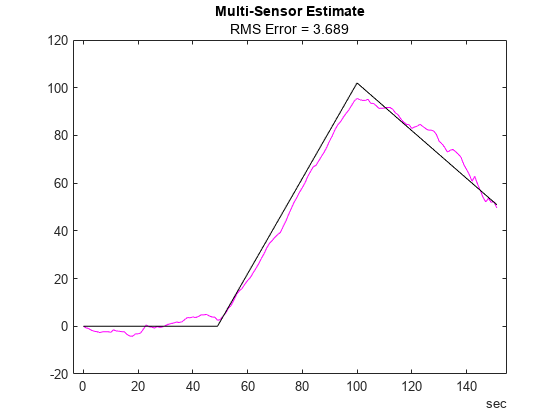
combinedOpts =  insOptions(SensorNamesSource="property", SensorNames={'VelocityWithBias', 'VelocityWithGM'});
sensorWithBias = exampleHelperVelocitySensorWithBias;
sensorWithGM = exampleHelperVelocitySensorWithGM;
filtCombined = insEKF(sensorWithBias, sensorWithGM, ...
    exampleHelperConstantVelocityMotion, combinedOpts);

% Combine the two sets of sensor measurements.
sensorData = synchronize(velBias, velGM, "first");
% Initialize the bias state with an estimate.
stateparts(filtCombined,  sensorWithBias, "Bias", ...
    mean(biasCalibrationData.VelocityWithBias));

mnCombined = tunernoise(filtCombined);
cfg4 =  tunerconfig(filtCombined, MaxIterations=tunerIters, Display='none');
combinedTunedNoise = tune(filtCombined, mnCombined, sensorData, ...
    groundTruth, cfg4);

estBoth = estimateStates(filtCombined, sensorData, combinedTunedNoise);
figure;
plot(estBoth.Time, estBoth.Position, 'm', groundTruth.Time, ...
    groundTruth.Position, 'k');
title("Multi-Sensor Estimate");
err = sqrt(mean((estBoth.Position - groundTruth.Position).^2));
subtitle("RMS Error = " + err);
snapnow;
Because the filter uses two sensors, both the bias and Gauss-Markov noise are observable. As a result, the filter obtains a more accurate velocity estimate and thus more accurate position estimate.
Conclusion
In this example, you learned the insEKF framework and how to customize sensor models used with the insEKF object. Implementing a custom motion model is almost the same process as implementing a new sensor, except that you inherit from the positioning.INSMotionModel interface class instead of the positioning.INSSensorModel interface class. Designing custom sensor fusion filters is straightforward with the insEKF framework and it is simple to build reusable sensors to use across projects.
References
[1] A Comparison between Different Error Modeling of MEMS Applied to GPS/INS Integrated Systems. A. Quinchia, G. Falco, E. Falletti, F. Dovis, C. Ferrer, Sensors 2013.