Implement Hardware-Efficient Complex Burst Matrix Solve Using QR Decomposition
This example shows how to implement a hardware-efficient least-squares solution to the complex-valued matrix equation AX=B using the Complex Burst Matrix Solve Using QR Decomposition block.
Define Matrix Dimensions
Specify the number of rows in matrices A and B, the number of columns in matrix A, and the number of columns in matrix B.
m = 50;  % Number of rows in matrices A and B
n = 10;  % Number of columns in matrix A
p = 1;   % Number of columns in matrix B
Generate Random Least-Squares Matrices
For this example, use the helper function complexRandomLeastSquaresMatrices to generate random matrices A and B for the least-squares problem AX=B. The matrices are generated such that the real and imaginary parts of the elements of A and B are between -1 and +1, and A has rank r.
rng('default')
r = 3;   % Rank of A
[A,B] = fixed.example.complexRandomLeastSquaresMatrices(m,n,p,r);
Select Fixed-Point Data Types
Use the helper function complexQRMatrixSolveFixedpointTypes to select fixed-point data types for input matrices A and B, and output X such that there is a low probability of overflow during the computation.
The real and imaginary parts of the elements of A and B are between -1 and 1, so the maximum possible absolute value of any element is sqrt(2).
max_abs_A = sqrt(2);  % Upper bound on max(abs(A(:))
max_abs_B = sqrt(2);  % Upper bound on max(abs(B(:))
precisionBits = 24;   % Number of bits of precision
T = fixed.complexQRMatrixSolveFixedpointTypes(m,n,max_abs_A,max_abs_B,precisionBits);
A = cast(A,'like',T.A);
B = cast(B,'like',T.B);
OutputType = fixed.extractNumericType(T.X);
Open the Model
model = 'ComplexBurstQRMatrixSolveModel';
open_system(model);
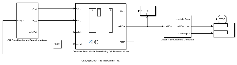
The Data Handler subsystem in this model takes complex matrices A and B as inputs. It sends rows of A and B to QR block using the AMBA AXI handshake protocol. The validIn signal indicates when data is available. The ready signal indicates that the block can accept the data. Transfer of data occurs only when both the validIn and ready signals are high. You can set a delay between the feeding in rows of A and B in the Data Handler to emulate the processing time of the upstream block. validIn remains high when rowDelay is set to 0 because this indicates the Data Handler always has data available.
Set Variables in the Model Workspace
Use the helper function setModelWorkspace to add the variables defined above to the model workspace. These variables correspond to the block parameters for the Complex Burst Matrix Solve Using QR Decomposition block.
numSamples = 1; % Number of sample matrices
rowDelay = 1; % Delay of clock cycles between feeding in rows of A and B
fixed.example.setModelWorkspace(model,'A',A,'B',B,'m',m,'n',n,'p',p,...
    'regularizationParameter',0,...
    'numSamples',numSamples,'rowDelay',rowDelay,'OutputType',OutputType);
Simulate the Model
out = sim(model);
Construct the Solution from the Output Data
The Complex Burst Matrix Solve Using QR Decomposition block outputs data one row at a time. When a result row is output, the block sets validOut to true. The rows of X are output in the order they are computed, last row first, so you must reconstruct the data to interpret the results. To reconstruct the matrix X from the output data, use the helper function matrixSolveModelOutputToArray.
X = fixed.example.matrixSolveModelOutputToArray(out.X,n,p,numSamples);
Verify the Accuracy of the Output
To evaluate the accuracy of the Complex Burst Matrix Solve Using QR Decomposition block, compute the relative error.
relative_error = norm(double(A*X - B))/norm(double(B)) %#ok<NOPTS>
relative_error =

   3.2836e-06