vecm
Convert vector autoregression (VAR) model to vector error-correction (VEC) model
Syntax
Description
Examples
Consider a VAR(2) model for the following seven macroeconomic series.
Gross domestic product (GDP)
GDP implicit price deflator
Paid compensation of employees
Nonfarm business sector hours of all persons
Effective federal funds rate
Personal consumption expenditures
Gross private domestic investment
Load the Data_USEconVECModel data set.
load Data_USEconVECModelFor more information on the data set and variables, enter Description at the command line.
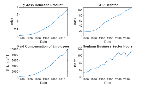
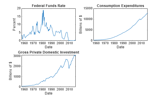
Determine whether the data needs to be preprocessed by plotting the series on separate plots.
figure;
subplot(2,2,1)
plot(FRED.Time,FRED.GDP);
title('Gross Domestic Product');
ylabel('Index');
xlabel('Date');
subplot(2,2,2)
plot(FRED.Time,FRED.GDPDEF);
title('GDP Deflator');
ylabel('Index');
xlabel('Date');
subplot(2,2,3)
plot(FRED.Time,FRED.COE);
title('Paid Compensation of Employees');
ylabel('Billions of $');
xlabel('Date');
subplot(2,2,4)
plot(FRED.Time,FRED.HOANBS);
title('Nonfarm Business Sector Hours');
ylabel('Index');
xlabel('Date');
figure;
subplot(2,2,1)
plot(FRED.Time,FRED.FEDFUNDS);
title('Federal Funds Rate');
ylabel('Percent');
xlabel('Date');
subplot(2,2,2)
plot(FRED.Time,FRED.PCEC);
title('Consumption Expenditures');
ylabel('Billions of $');
xlabel('Date');
subplot(2,2,3)
plot(FRED.Time,FRED.GPDI);
title('Gross Private Domestic Investment');
ylabel('Billions of $');
xlabel('Date');
Stabilize all series, except the federal funds rate, by applying the log transform. Scale the resulting series by 100 so that all series are on the same scale.
FRED.GDP = 100*log(FRED.GDP);
FRED.GDPDEF = 100*log(FRED.GDPDEF);
FRED.COE = 100*log(FRED.COE);
FRED.HOANBS = 100*log(FRED.HOANBS);
FRED.PCEC = 100*log(FRED.PCEC);
FRED.GPDI = 100*log(FRED.GPDI);
Create a VAR(2) model using the shorthand syntax. Specify the variable names.
Mdl = varm(7,2);
Mdl.SeriesNames = FRED.Properties.VariableNames;
Mdl is a varm model object. All properties containing NaN values correspond to parameters to be estimated given data.
Estimate the model using the entire data set and the default options.
EstMdl = estimate(Mdl,FRED.Variables)
EstMdl =
  varm with properties:

     Description: "AR-Stationary 7-Dimensional VAR(2) Model"
     SeriesNames: "GDP"  "GDPDEF"  "COE"  ... and 4 more
       NumSeries: 7
               P: 2
        Constant: [15.835 9.91375 -14.0917 ... and 4 more]'
              AR: {7×7 matrices} at lags [1 2]
           Trend: [7×1 vector of zeros]
            Beta: [7×0 matrix]
      Covariance: [7×7 matrix]
EstMdl is an estimated varm model object. It is fully specified because all parameters have known values.
Convert the estimated VAR(2) model to its equivalent VEC(1) model representation.
VECMdl = vecm(EstMdl)
VECMdl =
  vecm with properties:

             Description: "7-Dimensional Rank = 7 VEC(1) Model"
             SeriesNames: "GDP"  "GDPDEF"  "COE"  ... and 4 more
               NumSeries: 7
                    Rank: 7
                       P: 2
                Constant: [15.835 9.91375 -14.0917 ... and 4 more]'
              Adjustment: [7×7 matrix]
           Cointegration: [7×7 diagonal matrix]
                  Impact: [7×7 matrix]
   CointegrationConstant: [7×1 vector of NaNs]
      CointegrationTrend: [7×1 vector of NaNs]
                ShortRun: {7×7 matrix} at lag [1]
                   Trend: [7×1 vector of zeros]
                    Beta: [7×0 matrix]
              Covariance: [7×7 matrix]
VECMdl is a vecm model object.
Input Arguments
Output Arguments
Algorithms
Consider the m-dimensional VAR(p) model in difference equation notation.
yt is an m-by-1 vector of values corresponding to m response variables at time t, where t = 1,...,T.
c is the overall constant.
d is the overall time trend coefficient.
xt is a k-by-1 vector of values corresponding to k exogenous predictor variables.
β is an m-by-k matrix of regression coefficients.
εt is an m-by-1 vector of random Gaussian innovations, each with a mean of 0 and collectively an m-by-m covariance matrix Σ. For t ≠ s, εt and εs are independent.
Γj is an m-by-m matrix of autoregressive coefficients.
The equivalent VEC(p – 1) model using lag operator notation is
Lyt = yt – 1.
Π is an m-by-m impact matrix with a rank of r.
Φj is an m-by-m matrix of short-run coefficients
Version History
Introduced in R2017b