simulate
Simulate sample paths of threshold-switching dynamic regression model
Since R2021b
Description
Y = simulate(Mdl,numObs,Name,Value)simulate(Mdl,10,NumPaths=1000,Y0=Y0) simulates
1000 sample paths of length 10, and initializes the
dynamic component of each submodel by using the presample response data
Y0.
[
also returns the simulated innovation paths Y,E,StatePaths] = simulate(___)E and the simulated state
paths StatePaths, using any of the input argument combinations in the
previous syntaxes.
Examples
Suppose a data-generating process (DGP) is a two-state, self-exciting threshold autoregressive (SETAR) model for a 1-D response variable. Specify all parameter values (this example uses arbitrary values).
Create Fully Specified Model for DGP
Create a discrete threshold transition at level 0. Label the regimes to reflect the state of the economy:
When the threshold variable (currently unknown) is in , the economy is in a recession.
When the threshold variable is in , the economy is expanding.
t = 0;
tt = threshold(t,StateNames=["Recession" "Expansion"])
tt =
  threshold with properties:

          Type: 'discrete'
        Levels: 0
         Rates: []
    StateNames: ["Recession"    "Expansion"]
     NumStates: 2
tt is a fully specified threshold object that describes the switching mechanism of the threshold-switching model.
Assume the following univariate models describe the response process of the system:
Recession: , where .
Expansion: , where .
For each regime, use arima to create an AR model that describes the response process within the regime.
c1 = -1;
c2 = 1;
ar1 = 0.1;
ar2 = [0.3 0.2];
v1 = 1;
v2 = 4;

mdl1 = arima(Constant=c1,AR=ar1,Variance=v1,...
    Description="Recession State Model")
mdl1 =
  arima with properties:

     Description: "Recession State Model"
      SeriesName: "Y"
    Distribution: Name = "Gaussian"
               P: 1
               D: 0
               Q: 0
        Constant: -1
              AR: {0.1} at lag [1]
             SAR: {}
              MA: {}
             SMA: {}
     Seasonality: 0
            Beta: [1×0]
        Variance: 1

   ARIMA(1,0,0) Model (Gaussian Distribution)
mdl2 = arima(Constant=c2,AR=ar2,Variance=v2,...
    Description="Expansion State Model")
mdl2 =
  arima with properties:

     Description: "Expansion State Model"
      SeriesName: "Y"
    Distribution: Name = "Gaussian"
               P: 2
               D: 0
               Q: 0
        Constant: 1
              AR: {0.3 0.2} at lags [1 2]
             SAR: {}
              MA: {}
             SMA: {}
     Seasonality: 0
            Beta: [1×0]
        Variance: 4

   ARIMA(2,0,0) Model (Gaussian Distribution)
mdl1 and mdl2 are fully specified arima objects.
Store the submodels in a vector with order corresponding to the regimes in tt.StateNames.
mdl = [mdl1; mdl2];
Use tsVAR to create a TAR model from the switching mechanism tt and the state-specific submodels mdl.
Mdl = tsVAR(tt,mdl)
Mdl =
  tsVAR with properties:

         Switch: [1×1 threshold]
      Submodels: [2×1 varm]
      NumStates: 2
      NumSeries: 1
     StateNames: ["Recession"    "Expansion"]
    SeriesNames: "1"
     Covariance: []
Mdl.Submodels(2)
ans =
  varm with properties:

     Description: "AR-Stationary 1-Dimensional VAR(2) Model"
     SeriesNames: "Y1"
       NumSeries: 1
               P: 2
        Constant: 1
              AR: {0.3 0.2} at lags [1 2]
           Trend: 0
            Beta: [1×0 matrix]
      Covariance: 4
Mdl is a fully specified tsVAR object representing a univariate two-state TAR model. tsVAR stores specified arima submodels as varm objects.
Simulate Response Data from DGP
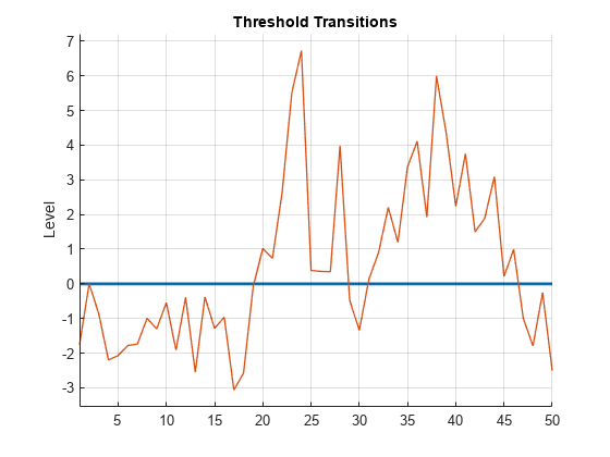
Generate one random response path of length 50 from the model. simulate assumes that the threshold variable is , which implies that the model is self-exciting.
rng(1); % For reproducibility
y = simulate(Mdl,50);
y is a 50-by-1 vector of one response path.
Plot the response path with the threshold by using ttplot.
figure
ttplot(Mdl.Switch,Data=y)
Consider the following logistic TAR (LSTAR) model for the annual, CPI-based, Canadian inflation rate series .
State 1: , where
State 2: , where
State 3: , where
The system is in state 1 when , the system is in state 2 when , and the system is in state 3 otherwise.
The transition function rate between states 1 and 2 is 3.5, and the transition function rate between states 2 and 3 is 1.5.
Create an LSTAR model representing .
t = [2 8];
tt = threshold([2 8],Type="logistic",Rates=[3.5 1.5]);

mdl1 = arima(Constant=-5,Variance=0.1);
mdl2 = arima(Constant=0,Variance=0.2);
mdl3 = arima(Constant=5,Variance=0.3);

Mdl = tsVAR(tt,[mdl1; mdl2; mdl3]);
Load the Canadian inflation and interest rate data set.
load Data_CanadaExtract the CPI-based inflation rate series.
INF_C = DataTable.INF_C;
numObs = length(INF_C);
Simulate ten paths from the model. Specify the threshold variable type and its data.
Y = simulate(Mdl,numObs,NumPaths=10,Type="exogenous",Z=INF_C);Y is a numObs-by-10 matrix of simulated paths. Each column represents an independently simulated path.
In a tiled layout, plot the threshold transitions with the data by using ttplot,and plot the simulated paths to one tile.
tiledlayout(2,1)
nexttile
ttplot(tt,Data=INF_C)
colorbar('off')
xticklabels(dates(xticks))
nexttile
plot(dates,Y)
grid on
axis tight
title("Simulations")
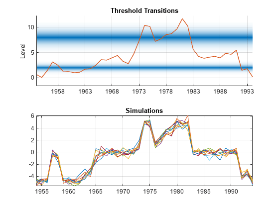
Y switches between submodels according to the value of the threshold variable INF_C. Mixing is evident for observations near thresholds, such as at the inflation rates of 1964 and 1978.
Consider the model for the annual, CPI-based, Canadian inflation rate series in Simulate Multiple Paths.
Create the LSTAR model for the series.
t = [2 8];
tt = threshold([2 8],Type="logistic",Rates=[3.5 1.5]);
mdl1 = arima(Constant=-5,Variance=0.1);
mdl2 = arima(Constant=0,Variance=0.2);
mdl3 = arima(Constant=5,Variance=0.3);
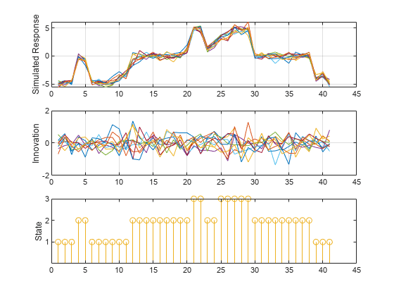
Mdl = tsVAR(tt,[mdl1; mdl2; mdl3]);Load the Canadian inflation and interest rate data set and extract the inflation rate series.
load Data_Canada
INF_C = DataTable.INF_C;
numObs = length(INF_C);
Simulate a length numObs path from the model. Specify the threshold variable type and its data. Return the innovations and states.
[y,e,s] = simulate(Mdl,numObs,NumPaths=10,Type="exogenous",Z=INF_C);

tiledlayout(3,1)
nexttile
plot(y);
ylabel("Simulated Response")
grid on

nexttile
plot(e)
ylabel('Innovation')
grid on

nexttile
stem(s)
ylabel('State')
yticks([1 2 3])
yticklabels(Mdl.StateNames)
This example shows how to initialize simulated paths from presample responses and initial states. The example uses arbitrary parameter values.
Fully Specify LSETAR Model
Consider the following 2-D LSETAR model.
State 1,
"Low": whereState 2 ,
"Med": whereState 3,
"High": whereThe system is in state 1 when , the system is in state 2 when , and the system is in state 3 otherwise.
The transition function is logistic. The transition rate from state 1 to 2 is 3.5, and the transition rate from state 1 to 3 is 1.5.
Create logistic threshold transitions at mid-levels -1 and 1 with rates 3.5 and 1.5, respectively. Label the states.
t = [-1 1];
r = [3.5 1.5];
stateNames = ["Low" "Med" "High"];
tt = threshold(t,Type="logistic",Rates=[3.5 1.5],StateNames=stateNames);
Create the VAR submodels by using varm. Store the submodels in a vector with order corresponding to the regimes in tt.StateNames.
% Constants (numSeries x 1 vectors)
C1 = [1; -1];
C2 = [2; -2];
C3 = [3; -3];

% Autoregression coefficients (numSeries x numSeries matrices)
AR1 = {};                            % 0 lags
AR2 = {[0.5 0.1; 0.5 0.5]};          % 1 lag
AR3 = {[0.25 0; 0 0] [0 0; 0.25 0]}; % 2 lags

% Innovations covariances (numSeries x numSeries matrices)
Sigma1 = [1 -0.1; -0.1 1];
Sigma2 = [2 -0.2; -0.2 2];
Sigma3 = [3 -0.3; -0.3 3];

% VAR Submodels
mdl1 = varm('Constant',C1,'AR',AR1,'Covariance',Sigma1);
mdl2 = varm('Constant',C2,'AR',AR2,'Covariance',Sigma2);
mdl3 = varm('Constant',C3,'AR',AR3,'Covariance',Sigma3);

mdl = [mdl1; mdl2; mdl3];
Create an LSETAR model from the switching mechanism tt and the state-specific submodels mdl. Label the series Y1 and Y2.
Mdl = tsVAR(tt,mdl,SeriesNames=["Y1" "Y2"])
Mdl =
  tsVAR with properties:

         Switch: [1×1 threshold]
      Submodels: [3×1 varm]
      NumStates: 3
      NumSeries: 2
     StateNames: ["Low"    "Med"    "High"]
    SeriesNames: ["Y1"    "Y2"]
     Covariance: []
Mdl is a fully specified tsVAR object representing a multivariate three-state LSETAR model. tsVAR object functions enable you to specify threshold variable characteristics and data.
Initialize Simulation from Presample Responses
Consider simulating 5 paths initialized from presample responses. Specify a numPreObs-by-numSeries-by-numPaths array of presample responses, where:
numPreObsis the number of presample responses per series and path. You must specify enough presample observations to initialize all AR components in the VAR models and the endogenous threshold variable. The largest AR component order is 2 and the threshold variable delay is 4, thereforesimulaterequiresnumPreObs=4presample observations per series and path.numSeries=2, the number of response series in the system.numPaths=5, the number of independent paths to simulate.
delay = 4;
numPaths = 5;
Y0 = zeros(delay,Mdl.NumSeries,numPaths);
for j = 2:numPaths
    Y0(:,:,j) = 10*j*ones(delay,Mdl.NumSeries);
end
Simulate 10 paths of length 100 from the LSETAR model from the presample. Specify the endogenous threshold variable and its delay, .
numObs = 100;
rng(1);
Y = simulate(Mdl,numObs,NumPaths=numPaths,Y0=Y0,Index=2,Delay=4);
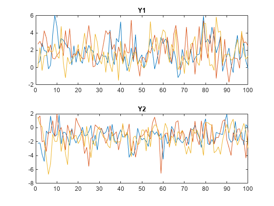
Y is a 100-by-2-by-5 array of simulate response paths. For example, Y(50,2,3) is the simulated response of path 3, of series Y2, at time point 50.
Plot the simulated paths for each variable on separate plots.
tiledlayout(2,1)
nexttile
plot(squeeze(Y(:,1,:)))
title("Y1")
nexttile
plot(squeeze(Y(:,2,:)))
title("Y2")
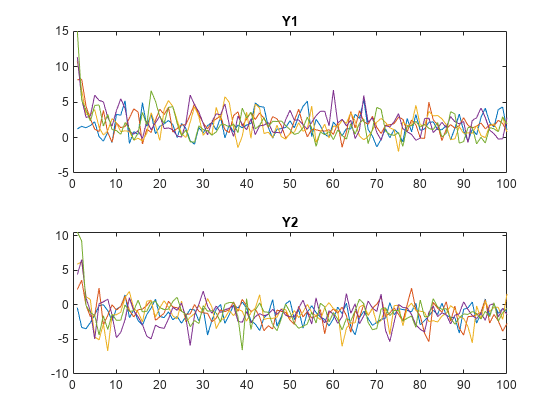
The system quickly settles regardless of the presample.
Initialize Simulation from States
Simulate three paths of length 100, where each of the three states initialize a path. Specify state indices for initialization, and specify the endogenous threshold variable and its delay.
S0 = 1:Mdl.NumStates;
numPaths = numel(S0);
Y = simulate(Mdl,numObs,NumPaths=numPaths,S0=S0,Index=2,Delay=4);
tiledlayout(2,1)
nexttile
plot(squeeze(Y(:,1,:)))
title("Y1")
nexttile
plot(squeeze(Y(:,2,:)))
title("Y2")
Consider including regression components for exogenous variables in each submodel of the threshold-switching dynamic regression model in Initialize Multivariate Model Simulation from Multiple Starting Conditions.
Fully Specify LSETAR Model
Create logistic threshold transitions at mid-levels -1 and 1 with rates 3.5 and 1.5, respectively. Label the states.
t = [-1 1];
r = [3.5 1.5];
stateNames = ["Low" "Med" "High"];
tt = threshold(t,Type="logistic",Rates=[3.5 1.5],StateNames=stateNames)
tt =
  threshold with properties:

          Type: 'logistic'
        Levels: [-1 1]
         Rates: [3.5000 1.5000]
    StateNames: ["Low"    "Med"    "High"]
     NumStates: 3
Assume the following VARX models describe the response processes of the system:
State 1: where
State 2: where
State 3: where
represents a single exogenous variable, represents two exogenous variables, and represents three exogenous variables. Store the submodels in a vector.
% Constants (numSeries x 1 vectors)
C1 = [1; -1];
C2 = [2; -2];
C3 = [3; -3];

% Regression coefficients (numSeries x numRegressors matrices)
Beta1 = [1; -1];            % 1 regressor
Beta2 = [2 2; -2 -2];       % 2 regressors
Beta3 = [3 3 3; -3 -3 -3];  % 3 regressors

% Autoregression coefficients (numSeries x numSeries matrices)
AR1 = {};
AR2 = {[0.5 0.1; 0.5 0.5]};
AR3 = {[0.25 0; 0 0] [0 0; 0.25 0]};

% Innovations covariances (numSeries x numSeries matrices)
Sigma1 = [1 -0.1; -0.1 1];
Sigma2 = [2 -0.2; -0.2 2];
Sigma3 = [3 -0.3; -0.3 3];

%VARX submodels
mdl1 = varm(Constant=C1,AR=AR1,Beta=Beta1,Covariance=Sigma1);
mdl2 = varm(Constant=C2,AR=AR2,Beta=Beta2,Covariance=Sigma2);
mdl3 = varm(Constant=C3,AR=AR3,Beta=Beta3,Covariance=Sigma3);

mdl = [mdl1; mdl2; mdl3];
Create an LSETAR model from the switching mechanism tt and the state-specific submodels mdl. Label the series Y1 and Y2.
Mdl = tsVAR(tt,mdl,SeriesNames=["Y1" "Y2"])
Mdl =
  tsVAR with properties:

         Switch: [1×1 threshold]
      Submodels: [3×1 varm]
      NumStates: 3
      NumSeries: 2
     StateNames: ["Low"    "Med"    "High"]
    SeriesNames: ["Y1"    "Y2"]
     Covariance: []
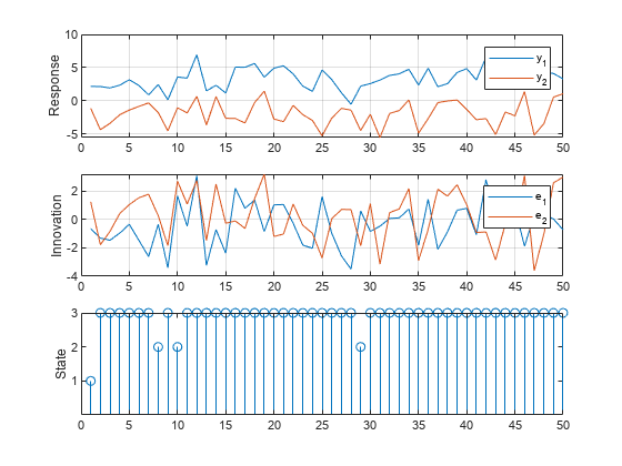
Simulate Data Ignoring Regression Component
If you do not supply exogenous data, simulate ignores the regression components in the submodels. Simulate a single path of responses, innovations, and states into a simulation horizon of length 50. Then plot each path separately.
rng(1); % For reproducibility
numObs = 50;
[Y,E,SP] = simulate(Mdl,numObs);

figure
tiledlayout(3,1)
nexttile
plot(Y)
ylabel("Response")
grid on
legend(["y_1" "y_2"])
nexttile
plot(E)
ylabel("Innovation")
grid on
legend(["e_1" "e_2"])
nexttile
stem(SP)
ylabel("State")
yticks([1 2 3])
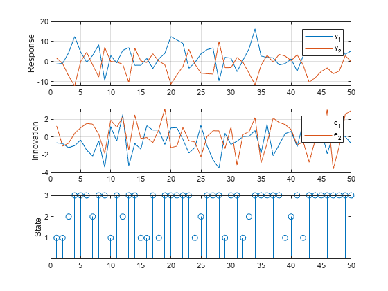
Simulate Data Including Regression Component
simulate requires exogenous data in order to generate random paths from the model. Simulate exogenous data for the three regressors by generating 50 random observations from the 3-D standard Gaussian distribution.
X = randn(50,3);
Generate one random response, innovation, and state path of length 50. Specify the simulated exogenous data for the submodel regression components. Plot the results.
rng(1); % Reset seed for comparison
[Y,E,SP] = simulate(Mdl,numObs,X=X);

figure
tiledlayout(3,1)
nexttile
plot(Y)
ylabel("Response")
grid on
legend(["y_1" "y_2"])
nexttile
plot(E)
ylabel("Innovation")
grid on
legend(["e_1" "e_2"])
nexttile
stem(SP)
ylabel("State")
yticks([1 2 3])
This example shows how to use Monte Carlo estimation to obtain an interval estimate of the threshold mid-level.
Consider a SETAR model for the real US GDP growth rate with AR(4) submodels. Suppose the threshold variable is (self exciting with 0 delay).
Create a discrete threshold transition at unknown mid-level . Label the states "Recession" and "Expansion".
tt = threshold(NaN,StateNames=["Recession" "Expansion"]);
For each state, create a partially specified AR(4) model with one coefficient at lag 4. Store the state submodels in a vector.
submdl = arima(ARLags=4);
mdl = [submdl; submdl];
Each submodel has an unknown, estimable lag 4 coefficient, model constant, and innovations variance.
Create a partially specified TAR model from the threshold transition and submodel vector.
Mdl = tsVAR(tt,mdl);
Create a fully specified threshold transition that has the same structure as tt, but set the mid-level to 0.
tt0 = threshold(0);
Load the US macroeconomic data set. Compute the real GDP growth rate as a percent.
load Data_USEconModel
rGDP = DataTimeTable.GDP./DataTimeTable.GDPDEF;
pRGDP = 100*price2ret(rGDP);
T = numel(pRGDP);
Fit the TAR to the real GDP rate series.
EstMdl = estimate(Mdl,tt0,pRGDP,Z=pRGDP,Type="exogenous");Simulate 100 response paths from the estimated model.
rng(100) % For reproducibility
numPaths= 100;
Y = simulate(EstMdl,T,NumPaths=numPaths,Z=pRGDP,Type="exogenous");
Fit the TAR model to each simulated response path. Specify the estimated threshold transition EstMdl.Switch to initialize the estimation procedure. For each path, store the estimated threshold transition mid-level.
tMC = nan(T,1);
for j = 1:numPaths
    EstMdlSim = estimate(Mdl,EstMdl.Switch,Y(:,j),Z=Y(:,j),Type="exogenous");
    tMC(j) = EstMdlSim.Switch.Levels;
end
tMC is a 100-by-1 vector representing a Monte Carlo sample of threshold transitions.
Obtain a 95% confidence interval on the true threshold transition by computing the 0.25 and .975 quantiles of the Monte Carlo sample.
tCI = quantile(tMC,[0.025 0.975])
tCI = 1×2

    0.5158    0.9810
A 95% confidence interval on the true threshold transition is (0.52%, 0.98%).
Input Arguments
Name-Value Arguments
Output Arguments
References
Version History
Introduced in R2021b