Create Regression Models with ARMA Errors

Default Regression Model with ARMA Errors

This example shows how to apply the shorthand regARIMA(p,D,q) syntax to specify the regression model with ARMA errors.

Specify the default regression model with ARMA(3,2) errors:

$$\begin{array}{l}{y}_t=c+X_t\beta +u_t\\ u_t=a_1{u}_{t-1}+a_2{u}_{t-2}+a_3{u}_{t-3}+{\epsilon }_t+b_1{\epsilon }_{t-1}+b_2{\epsilon }_{t-2}.\end{array}$$

Mdl = regARIMA(3,0,2)

Mdl = 
  regARIMA with properties:

     Description: "ARMA(3,2) Error Model (Gaussian Distribution)"
      SeriesName: "Y"
    Distribution: Name = "Gaussian"
       Intercept: NaN
            Beta: [1×0]
               P: 3
               Q: 2
              AR: {NaN NaN NaN} at lags [1 2 3]
             SAR: {}
              MA: {NaN NaN} at lags [1 2]
             SMA: {}
        Variance: NaN

The software sets each parameter to NaN, and the innovation distribution to Gaussian. The AR coefficients are at lags 1 through 3, and the MA coefficients are at lags 1 and 2.

Pass Mdl into estimate with data to estimate the parameters set to NaN. The regARIMA model sets Beta to [] and does not display it. If you pass a matrix of predictors ($$X_t$$) into estimate, then estimate estimates Beta. The estimate function infers the number of regression coefficients in Beta from the number of columns in $$X_t$$.

Tasks such as simulation and forecasting using simulate and forecast do not accept models with at least one NaN for a parameter value. Use dot notation to modify parameter values.

ARMA Error Model Without an Intercept

This example shows how to specify a regression model with ARMA errors without a regression intercept.

Specify the default regression model with ARMA(3,2) errors:

$$\begin{array}{l}{y}_t=X_t\beta +u_t\\ u_t=a_1{u}_{t-1}+a_2{u}_{t-2}+a_3{u}_{t-3}+{\epsilon }_t+b_1{\epsilon }_{t-1}+b_2{\epsilon }_{t-2}.\end{array}$$

Mdl = regARIMA('ARLags',1:3,'MALags',1:2,'Intercept',0)

Mdl = 
  regARIMA with properties:

     Description: "ARMA(3,2) Error Model (Gaussian Distribution)"
      SeriesName: "Y"
    Distribution: Name = "Gaussian"
       Intercept: 0
            Beta: [1×0]
               P: 3
               Q: 2
              AR: {NaN NaN NaN} at lags [1 2 3]
             SAR: {}
              MA: {NaN NaN} at lags [1 2]
             SMA: {}
        Variance: NaN

The software sets Intercept to 0, but all other parameters in Mdl are NaN values by default.

Since Intercept is not a NaN, it is an equality constraint during estimation. In other words, if you pass Mdl and data into estimate, then estimate sets Intercept to 0 during estimation.

You can modify the properties of Mdl using dot notation.

ARMA Error Model with Nonconsecutive Lags

This example shows how to specify a regression model with ARMA errors, where the nonzero ARMA terms are at nonconsecutive lags.

Specify the regression model with ARMA(8,4) errors:

$$\begin{array}{l}{y}_t=c+X_t\beta +u_t\\ u_t=a_1{u}_1+a_4{u}_4+a_8{u}_8+{\epsilon }_t+b_1{\epsilon }_{t-1}+b_4{\epsilon }_{t-4}.\end{array}$$

Mdl = regARIMA('ARLags',[1,4,8],'MALags',[1,4])

Mdl = 
  regARIMA with properties:

     Description: "ARMA(8,4) Error Model (Gaussian Distribution)"
      SeriesName: "Y"
    Distribution: Name = "Gaussian"
       Intercept: NaN
            Beta: [1×0]
               P: 8
               Q: 4
              AR: {NaN NaN NaN} at lags [1 4 8]
             SAR: {}
              MA: {NaN NaN} at lags [1 4]
             SMA: {}
        Variance: NaN

The AR coefficients are at lags 1, 4, and 8, and the MA coefficients are at lags 1 and 4. The software sets the interim lags to 0.

Pass Mdl and data into estimate. The software estimates all parameters that have the value NaN. Then estimate holds all interim lag coefficients to 0 during estimation.

Known Parameter Values for a Regression Model with ARMA Errors

This example shows how to specify values for all parameters of a regression model with ARMA errors.

Specify the regression model with ARMA(3,2) errors:

$$\begin{array}{l}{y}_t=X_t\left[\begin{array}{l}2.5\\ -0.6\end{array}\right]+u_t\\ u_t=0.7u_{t-1}-0.3u_{t-2}+0.1u_{t-3}+{\epsilon }_t+0.5{\epsilon }_{t-1}+0.2{\epsilon }_{t-2},\end{array}$$

where $${\epsilon }_t$$ is Gaussian with unit variance.

Mdl = regARIMA('Intercept',0,'Beta',[2.5; -0.6],...
    'AR',{0.7, -0.3, 0.1},'MA',{0.5, 0.2},'Variance',1)

Mdl = 
  regARIMA with properties:

     Description: "Regression with ARMA(3,2) Error Model (Gaussian Distribution)"
      SeriesName: "Y"
    Distribution: Name = "Gaussian"
       Intercept: 0
            Beta: [2.5 -0.6]
               P: 3
               Q: 2
              AR: {0.7 -0.3 0.1} at lags [1 2 3]
             SAR: {}
              MA: {0.5 0.2} at lags [1 2]
             SMA: {}
        Variance: 1

The parameters in Mdl do not contain NaN values, and therefore there is no need to estimate Mdl using estimate. However, you can simulate or forecast responses from Mdl using simulate or forecast.

Regression Model with ARMA Errors and t Innovations

This example shows how to set the innovation distribution of a regression model with ARMA errors to a t distribution.

Specify the regression model with ARMA(3,2) errors:

$$\begin{array}{l}{y}_t=X_t\left[\begin{array}{l}2.5\\ -0.6\end{array}\right]+u_t\\ u_t=0.7u_{t-1}-0.3u_{t-2}+0.1u_{t-3}+{\epsilon }_t+0.5{\epsilon }_{t-1}+0.2{\epsilon }_{t-2},\end{array}$$

where $${\epsilon }_t$$ has a t distribution with the default degrees of freedom and unit variance.

Mdl = regARIMA('Intercept',0,'Beta',[2.5; -0.6],...
    'AR',{0.7, -0.3, 0.1},'MA',{0.5, 0.2},'Variance',1,...
    'Distribution','t')

Mdl = 
  regARIMA with properties:

     Description: "Regression with ARMA(3,2) Error Model (t Distribution)"
      SeriesName: "Y"
    Distribution: Name = "t", DoF = NaN
       Intercept: 0
            Beta: [2.5 -0.6]
               P: 3
               Q: 2
              AR: {0.7 -0.3 0.1} at lags [1 2 3]
             SAR: {}
              MA: {0.5 0.2} at lags [1 2]
             SMA: {}
        Variance: 1

The default degrees of freedom is NaN. If you don't know the degrees of freedom, then you can estimate it by passing Mdl and the data to estimate.

Specify a $$t_5$$ distribution.

Mdl.Distribution = struct('Name','t','DoF',5)

Mdl = 
  regARIMA with properties:

     Description: "Regression with ARMA(3,2) Error Model (t Distribution)"
      SeriesName: "Y"
    Distribution: Name = "t", DoF = 5
       Intercept: 0
            Beta: [2.5 -0.6]
               P: 3
               Q: 2
              AR: {0.7 -0.3 0.1} at lags [1 2 3]
             SAR: {}
              MA: {0.5 0.2} at lags [1 2]
             SMA: {}
        Variance: 1

You can simulate or forecast responses from Mdl using simulate or forecast because Mdl is completely specified.

In applications, such as simulation, the software normalizes the random t innovations. In other words, Variance overrides the theoretical variance of the t random variable (which is DoF/(DoF - 2)), but preserves the kurtosis of the distribution.

Specify Regression Model with ARMA Errors Using Econometric Modeler App

In the Econometric Modeler app, you can specify the predictor variables in the regression component, and the error model lag structure and innovation distribution of a regression model with ARMA(p,q) errors, by following these steps. All specified coefficients are unknown but estimable parameters.

1. At the command line, open the Econometric Modeler app.

   econometricModeler

   Alternatively, open the app from the apps gallery (see Econometric Modeler).

2. In the Time Series pane, select the response time series to which the model will be fit.

3. On the Econometric Modeler tab, in the Models section, click the arrow to display the models gallery.

4. In the models gallery, in the Regression Models section, click RegARMA.

   The RegARMA Model Parameters dialog box appears.

   

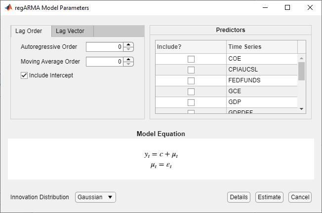
5. Choose the error model lag structure. To specify a regression model with ARMA(p,q) errors that includes all AR lags from 1 through p and all MA lags from 1 through q, use the Lag Order tab. For the flexibility to specify the inclusion of particular lags, use the Lag Vector tab. For more details, see Specifying Univariate Lag Operator Polynomials Interactively. Regardless of the tab you use, you can verify the model form by inspecting the equation in the Model Equation section.

6. In the Predictors section, choose at least one predictor variable by selecting the Include? check box for the time series.

For example, suppose you are working with the Data_USEconModel.mat data set and its variables are listed in the Time Series pane.

• To specify a regression model with AR(3) errors for the unemployment rate containing all consecutive AR lags from 1 through its order, Gaussian-distributed innovations, and the predictor variables COE, CPIAUCSL, FEDFUNDS, and GDP:

  1. In the Time Series pane, select the UNRATE time series.

  2. On the Econometric Modeler tab, in the Models section, click the arrow to display the models gallery.

  3. In the models gallery, in the Regression Models section, click RegARMA.

     .

  4. In the regARMA Model Parameters dialog box, on the Lag Order tab, set Autoregressive Order to 3.

  5. In the Predictors section, select the Include? check box for the COE, CPIAUCSL, FEDFUNDS, and GDP time series.

• To specify a regression model with MA(2) errors for the unemployment rate containing all MA lags from 1 through its order, Gaussian-distributed innovations, and the predictor variables COE and CPIAUCSL.

  1. In the Time Series pane, select the UNRATE time series.

  2. On the Econometric Modeler tab, in the Models section, click the arrow to display the models gallery.

  3. In the models gallery, in the Regression Models section, click RegARMA.

  4. In the regARMA Model Parameters dialog box, on the Lag Order tab, set Moving Average Order to 2.

  5. In the Predictors section, select the Include? check box for the COE and CPIAUCSL time series.

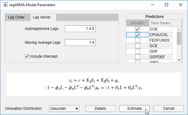
• To specify the regression model with ARMA(8,4) errors for the unemployment rate containing nonconsecutive lags

  $$\begin{array}{c}{y}_t=c+{\beta }_{1}CO{E}_t+{\beta }_{2}CPIAUCS{L}_t+u_t\\ \left(1-{\alpha }_{1}L-{\alpha }_4{L}^4-{\alpha }_8{L}^8\right)u_t=\left(1+b_{1}L+b_4{L}^4\right){\epsilon }_t\end{array},$$

  where ε_t is a series of IID Gaussian innovations:

  1. In the Time Series pane, select the UNRATE time series.

  2. On the Econometric Modeler tab, in the Models section, click the arrow to display the models gallery.

  3. In the models gallery, in the Regression Models section, click RegARMA.

  4. In the regARMA Model Parameters dialog box, click the Lag Vector tab:

     1. In the Autoregressive Lags box, type 1 4 8.

     2. In the Moving Average Lags box, type 1 4.

  5. In the Predictors section, select the Include? check box for the COE and CPIAUCSL time series.

  

• To specify a regression model with ARMA(3,2) errors for the unemployment rate containing all consecutive AR and MA lags through their respective orders, the predictor variables COE and CPIAUCSL, and t-distributed innovations:

  1. In the Time Series pane, select the UNRATE time series.

  2. On the Econometric Modeler tab, in the Models section, click the arrow to display the models gallery.

  3. In the models gallery, in the Regression Models section, click RegARMA.

  4. In the regARMA Model Parameters dialog box, click the Lag Order tab:

     1. Set Autoregressive Order to 3.

     2. Set Moving Average Order to 2.

  5. Click the Innovation Distribution button, then select t.

  6. In the Predictors section, select the Include? check box for the COE and CPIAUCSL time series.

  The degrees of freedom parameter of the t distribution is an unknown but estimable parameter.

After you specify a model, click Estimate to estimate all unknown parameters in the model.