Compare Generalized and Orthogonalized Impulse Response Functions
This example shows the differences between generalized and orthogonalized impulse response functions (IRFs) using the 3-D vector autoregression model containing the first two lags (VAR(2)) in [154], p. 78. The variables in the model represent the quarterly rates of fixed investment, disposable income, and consumption expenditures of Germany. The estimated model is
where and . The estimated covariance matrix of the innovations is
The VAR(2) model contains a constant, but because the IRF is the derivative of with respect to , the constant does not affect the IRF.
Create a cell vector containing the autoregressive coefficient matrices, and create the innovations covariance matrix.
AR1 = [-0.320  0.146  0.961;
        0.044 -0.153  0.289;
       -0.002  0.225 -0.264];
AR2 = [-0.161 0.115  0.934;
        0.050 0.019 -0.010;
        0.034 0.355 -0.022];
ar0 = {AR1 AR2};

InnovCov = [21.30 0.72 1.23;
             0.72 1.37 0.61;
             1.23 0.61 0.89]*1e-4;
Plot and compute the orthogonalized IRF in one armairf call by additionally returning the handle to the plotted graphics objects (the second output). Because no vector moving average (VMA) coefficients exist, specify an empty array ([]) for the second input argument.
[OrthoY,h] = armairf(ar0,[],'InnovCov',InnovCov);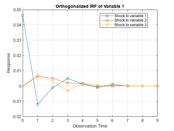
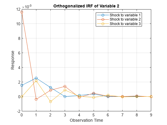
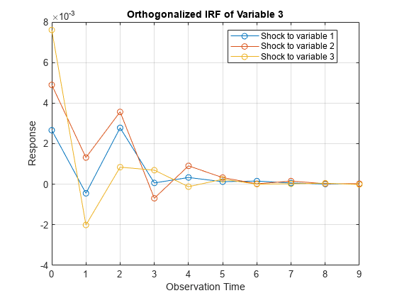
armairf returns separate figures, each containing IRFs of a variable in the system. Within a figure, armairf plots three separate line plots for the response of the variable to shocks to the three variables in the system at time 0. The orthogonalized impulse responses seem to fade after nine periods.
OrthoY is a 10-by-3-by-3 matrix of impulse responses. Each row corresponds to a time in the forecast horizon (0,...,9), each column corresponds to a variable receiving the shock at time 0, and each page corresponds to the IRF of a variable.
Plot and compute the generalized IRF.
[GenY,h] = armairf(ar0,[],'InnovCov',InnovCov,'Method','generalized');
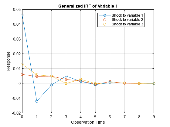
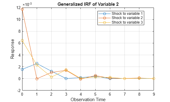
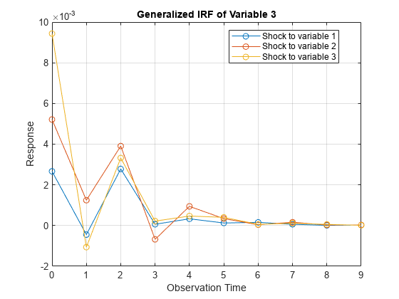
The generalized impulse responses seem to fade after nine periods, and appear to behave similarly to the orthogonalized impulse responses.
Display both sets of impulse responses.
for j = 1:3
    fprintf('Shock to Variable %d',j)
    table(squeeze(OrthoY(:,j,:)),squeeze(GenY(:,j,:)),'VariableNames',{'Orthogonalized',...
        'Generalized'})
end
Shock to Variable 1
ans=10×2 table
                 Orthogonalized                                 Generalized
    _________________________________________    _________________________________________

       0.046152      0.0015601      0.0026651       0.046152      0.0015601      0.0026651
       -0.01198      0.0025622    -0.00044488       -0.01198      0.0025622    -0.00044488
    -0.00098179      0.0012629      0.0027823    -0.00098179      0.0012629      0.0027823
      0.0049802     2.1799e-05     6.3661e-05      0.0049802     2.1799e-05     6.3661e-05
      0.0013726     0.00018127     0.00033187      0.0013726     0.00018127     0.00033187
    -0.00083369     0.00037736     0.00012609    -0.00083369     0.00037736     0.00012609
     0.00055287     1.0779e-05     0.00015701     0.00055287     1.0779e-05     0.00015701
     0.00027093     3.2276e-05     6.2713e-05     0.00027093     3.2276e-05     6.2713e-05
     3.7154e-05     5.1385e-05     9.3341e-06     3.7154e-05     5.1385e-05     9.3341e-06
      2.325e-05     1.0003e-05     2.8313e-05      2.325e-05     1.0003e-05     2.8313e-05
Shock to Variable 2
ans=10×2 table
                 Orthogonalized                                 Generalized
    _________________________________________    _________________________________________

              0         0.0116      0.0049001      0.0061514       0.011705      0.0052116
      0.0064026    -0.00035872      0.0013164      0.0047488    -1.4011e-05      0.0012454
      0.0050746     0.00088845      0.0035692      0.0048985      0.0010489      0.0039082
      0.0020934       0.001419    -0.00069114      0.0027385      0.0014093    -0.00067649
      0.0014919    -8.9823e-05     0.00090697      0.0016616     -6.486e-05     0.00094311
    -0.00043831     0.00048004     0.00032749    -0.00054552     0.00052606     0.00034138
      0.0011216     6.5734e-05     2.1313e-05      0.0011853     6.6585e-05      4.205e-05
     0.00010281     2.9385e-05     0.00015523       0.000138     3.3424e-05      0.0001622
    -3.2553e-05     0.00010201     2.6429e-05     -2.731e-05     0.00010795     2.7437e-05
     0.00018252    -5.2551e-06     2.6551e-05     0.00018399     -3.875e-06     3.0088e-05
Shock to Variable 3
ans=10×2 table
                 Orthogonalized                                 Generalized
    _________________________________________    _________________________________________

              0              0      0.0076083       0.013038       0.006466       0.009434
      0.0073116      0.0021988     -0.0020086      0.0058379      0.0023108     -0.0010618
      0.0031572    -0.00067127     0.00084299      0.0049047     0.00027687      0.0033197
     -0.0030985     0.00091269     0.00069346    -4.6882e-06      0.0014793     0.00021826
       0.001993     6.1109e-05    -0.00012102        0.00277     5.3838e-05     0.00046724
     0.00050636    -0.00010115     0.00024511    -5.4815e-05     0.00027437      0.0004034
    -0.00036814     0.00021062     3.6381e-06     0.00044188     0.00020705     5.8359e-05
     0.00028783    -2.6426e-05     2.3079e-05     0.00036206     3.0686e-06     0.00011696
     1.3105e-05     8.9361e-06     4.9558e-05     4.1567e-06     7.4706e-05     5.6331e-05
     1.6913e-05      2.719e-05    -1.1202e-05     0.00011501     2.2025e-05     1.2756e-05
If armairf shocks the first variable, then the impulse responses of all variables are equivalent between methods. The second and third columns suggest that the generalized and orthogonalized impulse responses are generally different. However, if InnovCov is diagonal, then both methods produce the same impulse responses.
Another difference between the two methods is that generalized impulse responses are invariant to the order of the variables, whereas orthogonalized impulse responses differ based on the variable order.