System Identification of FIR Filter Using LMS Algorithm
System identification is the process of identifying the coefficients of an unknown system using an adaptive filter. The general overview of the process is shown in System Identification –– Using an Adaptive Filter to Identify an Unknown System. The main components involved are:
The adaptive filter algorithm. In this example, set the
Methodproperty ofdsp.LMSFilterto'LMS'to choose the LMS adaptive filter algorithm.An unknown system or process to adapt to. In this example, the filter designed by
fircbandis the unknown system.Appropriate input data to exercise the adaptation process. For the generic LMS model, these are the desired signal and the input signal .
The objective of the adaptive filter is to minimize the error signal between the output of the adaptive filter and the output of the unknown system (or the system to be identified) . Once the error signal is minimized, the adapted filter resembles the unknown system. The coefficients of both the filters match closely.
Unknown System
Create a dsp.FIRFilter object that represents the system to be identified. Use the fircband function to design the filter coefficients. The designed filter is a lowpass filter constrained to 0.2 ripple in the stopband.
filt = dsp.FIRFilter;
filt.Numerator = fircband(12,[0 0.4 0.5 1],[1 1 0 0],[1 0.2],...
{'w' 'c'});
Pass the signal x to the FIR filter. The desired signal d is the sum of the output of the unknown system (FIR filter) and an additive noise signal n.
x = 0.1*randn(250,1);
n = 0.01*randn(250,1);
d = filt(x) + n;
Adaptive Filter
With the unknown filter designed and the desired signal in place, create and apply the adaptive LMS filter object to identify the unknown filter.
Preparing the adaptive filter object requires starting values for estimates of the filter coefficients and the LMS step size (mu). You can start with some set of nonzero values as estimates for the filter coefficients. This example uses zeros for the 13 initial filter weights. Set the InitialConditions property of dsp.LMSFilter to the desired initial values of the filter weights. For the step size, 0.8 is a good compromise between being large enough to converge well within 250 iterations (250 input sample points) and small enough to create an accurate estimate of the unknown filter.
Create a dsp.LMSFilter object to represent an adaptive filter that uses the LMS adaptive algorithm. Set the length of the adaptive filter to 13 taps and the step size to 0.8.
mu = 0.8;
lms = dsp.LMSFilter(13,'StepSize',mu)
lms =
dsp.LMSFilter with properties:
Method: 'LMS'
Length: 13
StepSizeSource: 'Property'
StepSize: 0.8000
LeakageFactor: 1
InitialConditions: 0
AdaptInputPort: false
WeightsResetInputPort: false
WeightsOutput: 'Last'
Show all properties
Pass the primary input signal x and the desired signal d to the LMS filter. Run the adaptive filter to determine the unknown system. The output y of the adaptive filter is the signal converged to the desired signal d thereby minimizing the error e between the two signals.
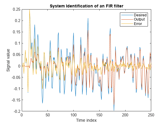
Plot the results. The output signal does not match the desired signal as expected, making the error between the two nontrivial.
[y,e,w] = lms(x,d);
plot(1:250, [d,y,e])
title('System Identification of an FIR filter')
legend('Desired','Output','Error')
xlabel('Time index')
ylabel('Signal value')
Compare the Weights
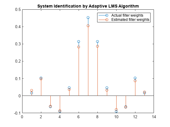
The weights vector w represents the coefficients of the LMS filter that is adapted to resemble the unknown system (FIR filter). To confirm the convergence, compare the numerator of the FIR filter and the estimated weights of the adaptive filter.
The estimated filter weights do not closely match the actual filter weights, confirming the results seen in the previous signal plot.
stem([(filt.Numerator).' w])
title('System Identification by Adaptive LMS Algorithm')
legend('Actual filter weights','Estimated filter weights',...
       'Location','NorthEast')
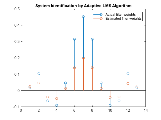
Changing the Step Size
As an experiment, change the step size to 0.2. Repeating the example with mu = 0.2 results in the following stem plot. The filters do not converge, and the estimated weights are not good approximations of the actual weights.
mu = 0.2;
lms = dsp.LMSFilter(13,'StepSize',mu);
[~,~,w] = lms(x,d);
stem([(filt.Numerator).' w])
title('System Identification by Adaptive LMS Algorithm')
legend('Actual filter weights','Estimated filter weights',...
       'Location','NorthEast')
Increase the Number of Data Samples
Increase the frame size of the desired signal. Even though this increases the computation involved, the LMS algorithm now has more data that can be used for adaptation. With 1000 samples of signal data and a step size of 0.2, the coefficients are aligned closer than before, indicating an improved convergence.
release(filt);
x = 0.1*randn(1000,1);
n = 0.01*randn(1000,1);
d = filt(x) + n;
[y,e,w] = lms(x,d);
stem([(filt.Numerator).' w])
title('System Identification by Adaptive LMS Algorithm')
legend('Actual filter weights','Estimated filter weights',...
       'Location','NorthEast')
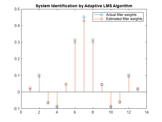
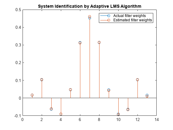
Increase the number of data samples further by inputting the data through iterations. Run the algorithm on 4000 samples of data, passed to the LMS algorithm in batches of 1000 samples over 4 iterations.
Compare the filter weights. The weights of the LMS filter match the weights of the FIR filter very closely, indicating a good convergence.
release(filt);
n = 0.01*randn(1000,1);
for index = 1:4
  x = 0.1*randn(1000,1);
  d = filt(x) + n;
  [y,e,w] = lms(x,d);
end
stem([(filt.Numerator).' w])
title('System Identification by Adaptive LMS Algorithm')
legend('Actual filter weights','Estimated filter weights',...
       'Location','NorthEast')
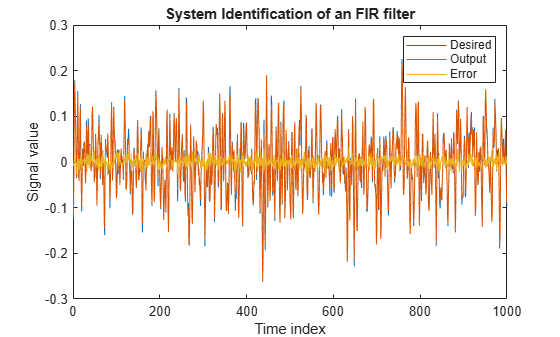
The output signal matches the desired signal very closely, making the error between the two close to zero.
plot(1:1000, [d,y,e])
title('System Identification of an FIR filter')
legend('Desired','Output','Error')
xlabel('Time index')
ylabel('Signal value')
See Also
Objects
Topics
- System Identification of FIR Filter Using Normalized LMS Algorithm
- Compare Convergence Performance Between LMS Algorithm and Normalized LMS Algorithm
References
[1] Hayes, Monson H., Statistical Digital Signal Processing and Modeling. Hoboken, NJ: John Wiley & Sons, 1996, pp.493–552.
[2] Haykin, Simon, Adaptive Filter Theory. Upper Saddle River, NJ: Prentice-Hall, Inc., 1996.