printToFigure
Description
printToFigure( prints the display window
of the scope)scope object to a new MATLAB® figure. The figure is visible by default.
Examples
Use the printToFigure function to print the spectrumAnalyzer object display window to a new MATLAB® figure.
Generate a chirp signal and use the spectrumAnalyzer object to display the spectrum of the chirp. This plot shows the default color and style settings of the spectrumAnalyzer object.
chirp = dsp.Chirp(SweepDirection="Bidirectional", ...
    TargetFrequency=2000, ...
    InitialFrequency=0,...
    TargetTime=400, ...
    SweepTime=400, ...
    SamplesPerFrame=1024, ...
    SampleRate=4000);
scope = spectrumAnalyzer(AveragingMethod="exponential",...
    ForgettingFactor=0,SampleRate=4000);
scope(chirp());

Change the background color and the axes color of the plot to "white". Set the font color and line color to "black".
scope.BackgroundColor = "white";
scope.AxesColor = "white";
scope.FontColor = "black";
scope.LineColor = "black";
show(scope)
release(scope)

Print the display of the chirp spectrum to a new MATLAB figure. The function returns a handle to the figure.
scopeFig = printToFigure(scope);

The handle to the figure scopeFig lets you modify the appearance and the behavior of the figure window.
Specify a figure name and change the size of the figure to 400-by-250 pixels.
scopeFig.Name="Spectrum of Chirp Signal";
scopeFig.NumberTitle="off";
scopeFig.Position=[1 1 400 250];

When printing to figure, you can make the figure invisible by setting the Visible argument to false.
scopeFig = printToFigure(scope,Visible=false);
Use the printToFigure function to print the dsp.ArrayPlot object display window to a new MATLAB® figure.
Create a dsp.ArrayPlot object.
scope=dsp.ArrayPlot;
Set ArrayPlot properties to display a Gaussian distribution.
scope.YLimits = [-0.1 1.1];
scope.XOffset = -2.5;
scope.SampleIncrement = 0.1;
scope.Title = "Gaussian distribution";
scope.XLabel = "X";
scope.YLabel = "f(X)";
Plot the Gaussian distribution.
scope(exp(-(-2.5:.1:2.5) .* (-2.5:.1:2.5))');

Change the background color and the axes color of the plot to "white". Set the font color to "black" and the line color to "blue".
scope.BackgroundColor = "white";
scope.AxesColor = "white";
scope.FontColor = "black";
scope.LineColor = "blue";
show(scope)
release(scope)

Print the display of the Gaussian distribution to a new MATLAB figure. The function returns a handle to the figure.
scopeFig = printToFigure(scope);

The handle to the figure scopeFig lets you modify the appearance and the behavior of the figure window.
Specify a figure name and change the size of the figure to 400-by-250 pixels.
scopeFig.Name="Gaussian Distribution";
scopeFig.NumberTitle="off";
scopeFig.Position=[1 1 400 250];

When printing to figure, you can make the figure invisible by setting the Visible argument to false.
scopeFig = printToFigure(scope,Visible=false);
Use the printToFigure function to print the timescope object display window to a new MATLAB® figure.
The timescope object requires one of these products:
DSP System Toolbox™
Navigation Toolbox™
Sensor Fusion and Tracking Toolbox™
View a sine wave on the time scope. This plot shows the default color and style settings of the timescope object.
f = 100;
fs = 1000;
swv = sin(2.*pi.*f.*(0:1/fs:1-1/fs)).';
scope = timescope(SampleRate=fs,...
    TimeSpanSource="property", ...
    TimeSpan=1);
scope(swv);

Change the background color and the axes color of the plot to "white". Set the font color to "black" and the line color to "blue".
scope.BackgroundColor = "white";
scope.AxesColor = "white";
scope.FontColor = "black";
scope.LineColor = "blue";
show(scope)
release(scope)

Print the display of the sine wave to a new MATLAB figure. The function returns a handle to the figure.
scopeFig = printToFigure(scope);

The handle to the figure scopeFig lets you modify the appearance and the behavior of the figure window.
Specify a figure name and change the size of the figure to 400-by-250 pixels.
scopeFig.Name="Sine Wave Signal";
scopeFig.NumberTitle="off";
scopeFig.Position=[1 1 400 250];

When printing to figure, you can make the figure invisible by setting the Visible argument to false.
scopeFig = printToFigure(scope,Visible=false);
Use the printToFigure function to print the dsp.DynamicFilterVisualizer object display window to a new MATLAB® figure.
Create a dsp.DynamicFilterVisualizer object.
dfv = dsp.DynamicFilterVisualizer(YLimits=[-120 10]);
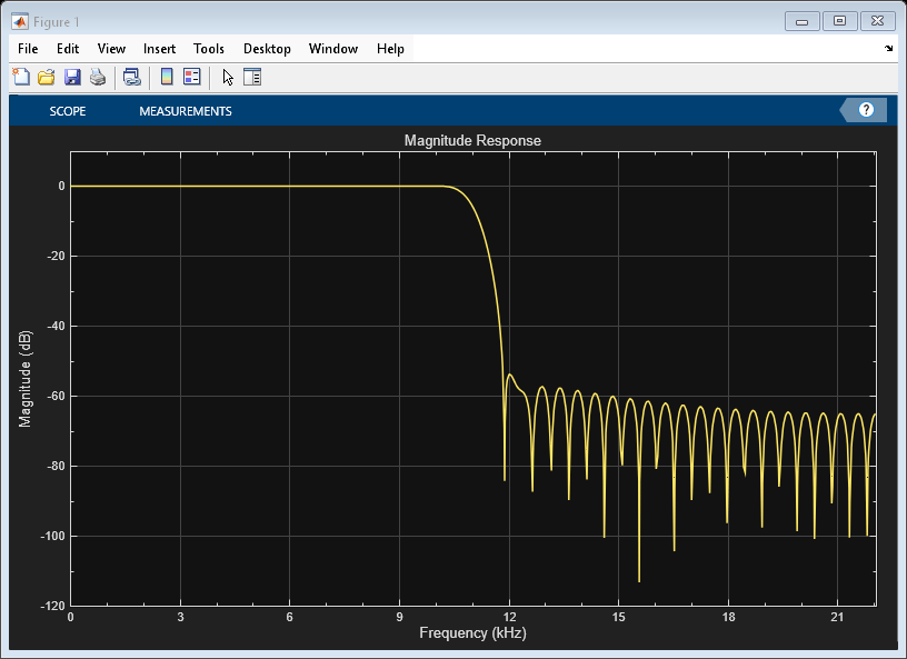
Design FIR filter with varying cutoff frequencies ranging from 0.1 to 0.5. Plot the magnitude response of the filter using the Dynamic Filter Visualizer.
for k = 0.1:0.001:0.5
    b = fir1(90, k);
    dfv(b,1);
end

Change the background color and the axes color of the plot to "white". Set the font color to "black" and the line color to "blue".
dfv.BackgroundColor = "white";
dfv.AxesColor = "white";
dfv.FontColor = "black";
dfv.LineColor = "blue";
show(dfv)
release(dfv)

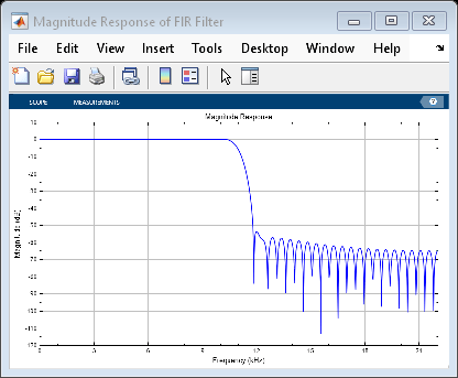
Print the display of the magnitude response to a new MATLAB figure. The function returns a handle to the figure.
scopeFig = printToFigure(dfv);

The handle to the figure scopeFig lets you modify the appearance and the behavior of the figure window.
Specify a figure name and change the size of the figure to 400-by-250 pixels.
scopeFig.Name="Magnitude Response of FIR Filter";
scopeFig.NumberTitle="off";
scopeFig.Position=[1 1 400 250];

When printing to figure, you can make the figure invisible by setting the Visible argument to false.
scopeFig = printToFigure(dfv,Visible=false);
Input Arguments
Scope object whose display the function prints to a MATLAB figure, specified as one of the following:
spectrumAnalyzerobjectdsp.ArrayPlotobjecttimescopeobjectdsp.DynamicFilterVisualizerobject
Flag to show the MATLAB figure, specified as true or
false.
Data Types: logical
Output Arguments
Handle to the MATLAB figure, returned as a Figure object. For more
information on the properties of this object, see Figure.
Version History
Introduced in R2023b
MATLAB Command
You clicked a link that corresponds to this MATLAB command:
Run the command by entering it in the MATLAB Command Window. Web browsers do not support MATLAB commands.
웹사이트 선택
번역된 콘텐츠를 보고 지역별 이벤트와 혜택을 살펴보려면 웹사이트를 선택하십시오. 현재 계신 지역에 따라 다음 웹사이트를 권장합니다:
또한 다음 목록에서 웹사이트를 선택하실 수도 있습니다.
사이트 성능 최적화 방법
최고의 사이트 성능을 위해 중국 사이트(중국어 또는 영어)를 선택하십시오. 현재 계신 지역에서는 다른 국가의 MathWorks 사이트 방문이 최적화되지 않았습니다.
미주
- América Latina (Español)
- Canada (English)
- United States (English)
유럽
- Belgium (English)
- Denmark (English)
- Deutschland (Deutsch)
- España (Español)
- Finland (English)
- France (Français)
- Ireland (English)
- Italia (Italiano)
- Luxembourg (English)
- Netherlands (English)
- Norway (English)
- Österreich (Deutsch)
- Portugal (English)
- Sweden (English)
- Switzerland
- United Kingdom (English)