Compress Deep Learning Network for Battery State of Charge Estimation

Since R2024b

Step 4 of 7 in Battery State of Charge Estimation Using Deep Learning

This example shows how to compress a neural network for predicting the state of charge of a battery using projection.

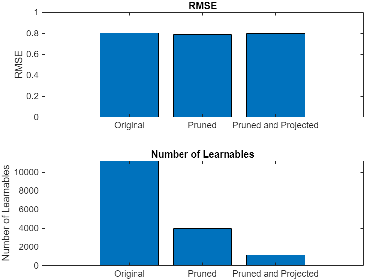
Neural networks can take up large amounts of memory. If you have a memory requirement for your network, for example because you want to embed it into a resource-constrained hardware target, then you might need to compress your model to meet the requirement. Compressing a network reduces the size of the network in memory whilst aiming to maintain overall performance. For example, in the following image, you can see an example where compressing a network using first pruning and then projection reduces the number of learnables and has little impact on the root mean squared error (RMSE).

This example is the fourth step in a series of examples that take you through a battery state of charge estimation workflow. You can run each step independently or work through the steps in order. This example follows the Train Deep Learning Network for Battery State of Charge Estimation example. For more information about the full workflow, see Battery State of Charge Estimation Using Deep Learning.

Load the test data. If you have run the previous step, then load the data you saved in the previous step. Otherwise, the example prepares the data as shown in Prepare Data for Battery State of Charge Estimation Using Deep Learning.

if ~exist("XTrain","var") || ~exist("YTrain","var") || ~exist("XVal","var") || ~exist("YVal","var")
    [XTrain,YTrain,XVal,YVal] = prepareBSOCData;
end

Load a pretrained network. If you have run the previous step, then the example uses your trained network. Otherwise, load a pretrained network. This network has been trained using the steps shown in Train Deep Learning Network for Battery State of Charge Estimation.

if ~exist("recurrentNet")
    load("pretrainedBSOCNetwork.mat")
end

This example requires the Deep Learning Toolbox™ Model Quantization Library support package. This support package is a free add-on that you can download using the Add-On Explorer.

Explore Compression Levels

Projection is a layer-wise compression technique that replaces a large layer with one or more layers with a smaller total number of parameters.

The compressNetworkUsingProjection function uses principal component analysis (PCA) to identify the subspace of learnable parameters that result in the highest variance in neuron activations. Then, the function projects the layer onto this lower-dimensional subspace and performs the layer operation within the lower-dimensional space.

The PCA step can be computationally intensive. If you expect to compress the same network multiple times (for example, when exploring different levels of compression), then perform the PCA step first using the neuronPCA function, then pass the output of this function to the compressNetworkUsingProjection function as an input argument.

The neuronPCA function analyzes the network activations using a data set of training data, or a representative subset thereof. This analysis requires only the predictors of the training data to compute the network activations. It does not require the training targets.

Create a mini-batch queue containing the training data.

mbq = minibatchqueue(...
    arrayDatastore(XTrain',IterationDimension=1,OutputType="same",ReadSize=numel(XTrain)), ...
    MiniBatchSize=32, ...
    MiniBatchFormat="TCB", ...
    MiniBatchFcn=@(X) cat(3,X{:}));

Create the neuronPCA object. To view information about the steps of the neuron PCA algorithm, set the VerbosityLevel option to "steps".

npca = neuronPCA(recurrentNet,mbq,VerbosityLevel="steps");

Using solver mode "direct".
Computing covariance matrices for activations connected to: "lstm_1/in","lstm_1/out","lstm_2/in","lstm_2/out","fc/in","fc/out"
Computing eigenvalues and eigenvectors for activations connected to: "lstm_1/in","lstm_1/out","lstm_2/in","lstm_2/out","fc/in","fc/out"
neuronPCA analyzed 3 layers: "lstm_1","lstm_2","fc"

View the properties of the neuronPCA object.

npca

npca = 
  neuronPCA with properties:

                  LayerNames: ["lstm_1"    "lstm_2"    "fc"]
      ExplainedVarianceRange: [0 1]
    LearnablesReductionRange: [0.8525 0.9884]
            InputEigenvalues: {[3×1 double]  [256×1 double]  [128×1 double]}
           InputEigenvectors: {[3×3 double]  [256×256 double]  [128×128 double]}
           OutputEigenvalues: {[256×1 double]  [128×1 double]  [1.0907]}
          OutputEigenvectors: {[256×256 double]  [128×128 double]  [1]}

The explained variance of a network details how well the space of network activations can capture the underlying features of the data. To explore different amounts of compression, iterate over different values of the ExplainedVarianceGoal option of the compressNetworkUsingProjection function and compare the results. Alternatively, you can sweep over the learnable reduction goal.

numValues = 10;
explainedVarGoal = 1 - [0 logspace(-3,0,numValues)];
explainedVariance = zeros(1,numValues);
learnablesReduction = zeros(1,numValues);
valRMSE = zeros(1,numValues);

for i = 1:numValues
    varianceGoal = explainedVarGoal(i);

    [trialNetwork,info] = compressNetworkUsingProjection(recurrentNet,npca, ...
        ExplainedVarianceGoal=varianceGoal, ...
        VerbosityLevel="off");

    explainedVariance(i) = info.ExplainedVariance;
    learnablesReduction(i) = info.LearnablesReduction;
    valRMSE(i) = testnet(trialNetwork,XVal,YVal,"rmse");
end

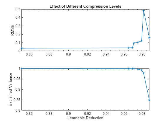
Plot the RMSE of the compressed networks against their explained variance goal.

figure
tiledlayout("flow")
nexttile
plot(learnablesReduction,valRMSE,'*-')
ylabel("RMSE")
xscale("log")
title("Effect of Different Compression Levels")

nexttile
plot(learnablesReduction,explainedVariance,'*-')
ylim([0.8 1])
ylabel("Explained Variance")
xlabel("Learnable Reduction")
xscale("log")

The graph shows that an increase in learnable reduction has a corresponding increase in RMSE (decrease in accuracy). A learnable reduction value of around 96% shows a good compromise between the amount of compression and RMSE.

If you require more compression than that, specify a higher learnables reduction and then retrain the model after projection to fine-tune it. Fine-tuning the model can regain significant amounts of accuracy lost in the projection step.

Compress Network Using Projection

Compress the network using the neuronPCA object with a learnable reduction goal of 96% using the compressNetworkUsingProjection function. To ensure that the projected network supports library-free code generation, specify that the projected layers are unpacked.

recurrentNetProjected = compressNetworkUsingProjection(recurrentNet,npca, ...
    LearnablesReductionGoal=0.96, ...
    UnpackProjectedLayers=true);

Compressed network has 96.0% fewer learnable parameters.
Projection compressed 3 layers: "lstm_1","lstm_2","fc"

Compare Original and Compressed Networks

Evaluate the projected network´s performance on the test data set.

RMSE = testnet(recurrentNet,XVal,YVal,"rmse")

RMSE = 
0.0333

RMSEProjected = testnet(recurrentNetProjected,XVal,YVal,"rmse")

RMSEProjected = 
0.0360

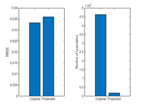
Compressing the network has negligible impact on the RMSE of the predictions.

Compare the error and model size of the original and compressed networks.

learnables = numLearnables(recurrentNet);
learnablesProjected = numLearnables(recurrentNetProjected);
% Plot root mean squared error.
figure
tiledlayout(1,2)
nexttile
bar([RMSE RMSEProjected])
xticklabels(["Original" "Projected"])
ylabel("RMSE")

% Plot numbers of learnables.
nexttile
bar([learnables learnablesProjected])
xticklabels(["Original" "Projected"])
ylabel("Number of Learnables")

Compared to the original network, the projected network has a significantly smaller size and has only slightly less prediction accuracy. Smaller networks typically have a reduced inference time.

Test Compressed Model Predictions

Test the model predictions on unseen test data. Specify the temperature range to test over. This example tests the model on data at the temperatures -10, 0, 10, and 25 degrees Celsius.

temp = ["n10" "0" "10" "25"];

Use the minibatchpredict function to generate predictions for each temperature.

dataTrue = [];
YPred = [];
RMSE = [];

for i = 1:4

% Load test data.
filename = "BSOC_" + temp(i) + "_degrees.mat";
testFile = fullfile("BSOCTestingData",filename);
dataTrue{i} = load(testFile);

load("BSOCTrainingMaxMinStats.mat")
dataTrue{i}.X = rescale(dataTrue{i}.X,InputMin=minX,InputMax=maxX);

% Generate predictions.
YPred{i} = minibatchpredict(recurrentNet,dataTrue{i}.X);
YPredCompressed{i} = minibatchpredict(recurrentNetProjected,dataTrue{i}.X);

end

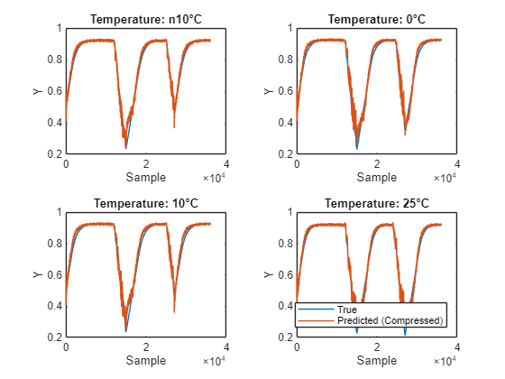
Plot the predictions from each network and the measured values. You can see that the compressed model predicts the true value well.

figure
tiledlayout("flow")
for i = 1:4
    nexttile
plot(dataTrue{i}.Y); 
hold on;
plot(YPredCompressed{i});
hold off
xlabel("Sample")
ylabel("Y")
if i == 4
legend(["True" "Predicted (Compressed)"],Location="southeast")
end
title("Temperature: " + temp(i) + "°C")
end

Save Network

Save the compressed neural network.

useCompressedNetwork = true;

if useCompressedNetwork
    recurrentNet = recurrentNetProjected;
end

Supporting Functions

numLearnables

The numLearnables function receives a network as input and returns the total number of learnables in that network.

function N = numLearnables(net)
    N = 0;
    for i = 1:size(net.Learnables,1)
        N = N + numel(net.Learnables.Value{i});
    end
end

Next step: Test Deep Learning Network for Battery State of Charge Estimation. You can also open the next example using the openExample function.

openExample("deeplearning_shared/TestModelForBatteryStateOfChargeEstimationExample")