Classify Text Data Using Custom Training Loop
This example shows how to classify text data using a deep learning bidirectional long short-term memory (BiLSTM) network with a custom training loop.
When training a deep learning network using the trainnet function, if trainingOptions does not provide the options you need (for example, a custom solver), then you can define your own custom training loop using automatic differentiation. For an example showing how to classify text data using the trainnet function, see Classify Text Data Using Deep Learning.
This example trains a network to classify text data with the stochastic gradient descent algorithm (without momentum).
Import Data
Import the factory reports data. This data contains labeled textual descriptions of factory events. To import the text data as strings, specify the text type to be "string".
filename = "factoryReports.csv";
data = readtable(filename,TextType="string");
head(data)
                                 Description                                       Category          Urgency          Resolution         Cost
    _____________________________________________________________________    ____________________    ________    ____________________    _____

    "Items are occasionally getting stuck in the scanner spools."            "Mechanical Failure"    "Medium"    "Readjust Machine"         45
    "Loud rattling and banging sounds are coming from assembler pistons."    "Mechanical Failure"    "Medium"    "Readjust Machine"         35
    "There are cuts to the power when starting the plant."                   "Electronic Failure"    "High"      "Full Replacement"      16200
    "Fried capacitors in the assembler."                                     "Electronic Failure"    "High"      "Replace Components"      352
    "Mixer tripped the fuses."                                               "Electronic Failure"    "Low"       "Add to Watch List"        55
    "Burst pipe in the constructing agent is spraying coolant."              "Leak"                  "High"      "Replace Components"      371
    "A fuse is blown in the mixer."                                          "Electronic Failure"    "Low"       "Replace Components"      441
    "Things continue to tumble off of the belt."                             "Mechanical Failure"    "Low"       "Readjust Machine"         38
The goal of this example is to classify events by the label in the Category column. To divide the data into classes, convert these labels to categorical.
data.Category = categorical(data.Category);
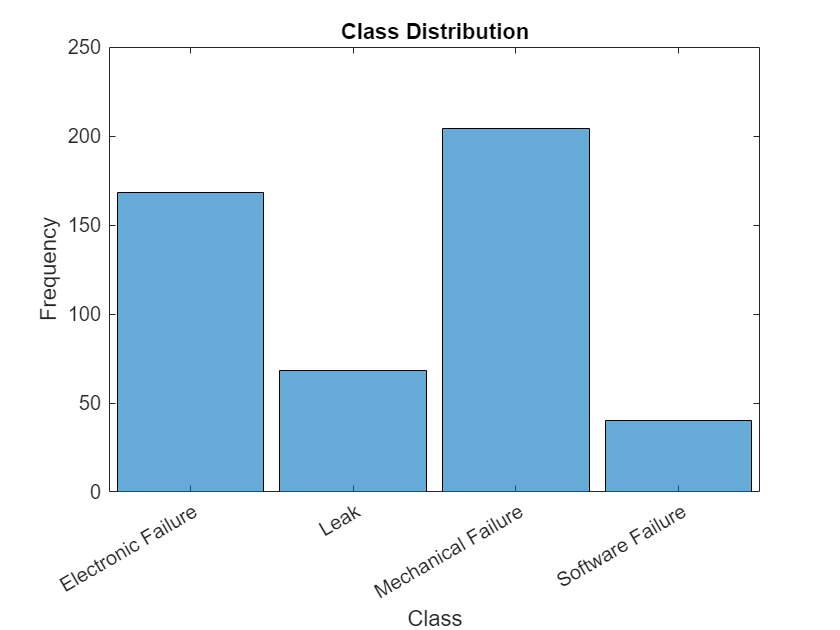
View the distribution of the classes in the data using a histogram.
figure
histogram(data.Category);
xlabel("Class")
ylabel("Frequency")
title("Class Distribution")
The next step is to partition it into sets for training and validation. Partition the data into a training partition and a held-out partition for validation and testing. Specify the holdout percentage to be 20%.
cvp = cvpartition(data.Category,Holdout=0.2);
dataTrain = data(training(cvp),:);
dataValidation = data(test(cvp),:);
Extract the text data and labels from the partitioned tables.
textDataTrain = dataTrain.Description;
textDataValidation = dataValidation.Description;
TTrain = dataTrain.Category;
TValidation = dataValidation.Category;
To check that you have imported the data correctly, visualize the training text data using a word cloud.
figure
wordcloud(textDataTrain);
title("Training Data")
View the number of classes.
classes = categories(TTrain);
numClasses = numel(classes)
numClasses =
4
Preprocess Text Data
Create a function that tokenizes and preprocesses the text data. The function preprocessText, listed at the end of the example, performs these steps:
Tokenize the text using
tokenizedDocument.Convert the text to lowercase using
lower.Erase the punctuation using
erasePunctuation.
Preprocess the training data and the validation data using the preprocessText function.
documentsTrain = preprocessText(textDataTrain);
documentsValidation = preprocessText(textDataValidation);
View the first few preprocessed training documents.
documentsTrain(1:5)
ans =
  5×1 tokenizedDocument:

     9 tokens: items are occasionally getting stuck in the scanner spools
    10 tokens: there are cuts to the power when starting the plant
     5 tokens: fried capacitors in the assembler
     4 tokens: mixer tripped the fuses
     8 tokens: things continue to tumble off of the belt
Create a single datastore that contains both the training documents and the labels by creating arrayDatastore objects, then combining them using the combine function.
dsDocumentsTrain = arrayDatastore(documentsTrain,OutputType="cell");
dsTTrain = arrayDatastore(TTrain,OutputType="cell");
dsTrain = combine(dsDocumentsTrain,dsTTrain);
Create an datastore for the validation data using the same steps.
dsDocumentsValidation = arrayDatastore(documentsValidation,OutputType="cell");
dsTValidation = arrayDatastore(TValidation,OutputType="cell");
dsValidation = combine(dsDocumentsValidation,dsTValidation);
Create Word Encoding
To input the documents into a BiLSTM network, use a word encoding to convert the documents into sequences of numeric indices.
To create a word encoding, use the wordEncoding function.
enc = wordEncoding(documentsTrain)
enc =
  wordEncoding with properties:

      NumWords: 425
    Vocabulary: ["items"    "are"    "occasionally"    "getting"    "stuck"    "in"    "the"    "scanner"    "spools"    "there"    "cuts"    "to"    "power"    "when"    "starting"    "plant"    "fried"    "capacitors"    …    ] (1×425 string)
Define Network
Define the BiLSTM network architecture. To input sequence data into the network, include a sequence input layer and set the input size to 1. Next, include a word embedding layer of dimension 25 and the same number of words as the word encoding. Next, include a BiLSTM layer and set the number of hidden units to 40. To use the BiLSTM layer for a sequence-to-label classification problem, set the output mode to "last". Finally, add a fully connected layer with the same size as the number of classes, and a softmax layer.
inputSize = 1;
embeddingDimension = 25;
numHiddenUnits = 40;

numWords = enc.NumWords;

layers = [
    sequenceInputLayer(inputSize)
    wordEmbeddingLayer(embeddingDimension,numWords)
    bilstmLayer(numHiddenUnits,OutputMode="last")
    fullyConnectedLayer(numClasses)
    softmaxLayer]
layers =
5×1 Layer array with layers:
1 '' Sequence Input Sequence input with 1 dimensions
2 '' Word Embedding Layer Word embedding layer with 25 dimensions and 425 unique words
3 '' BiLSTM BiLSTM with 40 hidden units
4 '' Fully Connected 4 fully connected layer
5 '' Softmax softmax
Convert the layer array to a dlnetwork object.
net = dlnetwork(layers)
net =
  dlnetwork with properties:

         Layers: [5×1 nnet.cnn.layer.Layer]
    Connections: [4×2 table]
     Learnables: [6×3 table]
          State: [2×3 table]
     InputNames: {'sequenceinput'}
    OutputNames: {'softmax'}
    Initialized: 1

  View summary with summary.
Define Model Loss Function
Create the model loss function. The modelLoss function takes a dlnetwork object net, a mini-batch of input data X with corresponding target labels T and returns the gradients of the loss with respect to the learnable parameters in net, and the loss. To compute the gradients automatically, use the dlgradient function.
function [loss,gradients] = modelLoss(net,X,T)

Y = forward(net,X);
loss = crossentropy(Y,T);
gradients = dlgradient(loss,net.Learnables);

end
Define SGD Function
Create the function sgdStep that takes the parameters and the gradients of the loss with respect to the parameters, and returns the updated parameters using the stochastic gradient descent algorithm, expressed as , where is the iteration number, is the learning rate, and denotes the gradients (the derivatives of the loss with respect to the learnable parameters).
function parameters = sgdStep(parameters,gradients,learnRate)

parameters = parameters - learnRate .* gradients;

end
Defining a custom update function is not a necessary step for custom training loops. Alternatively, you can use built in update functions like sgdmupdate, adamupdate, and rmspropupdate.
Specify Training Options
Train for 300 epochs with a mini-batch size of 64 and a learning rate of 0.1.
numEpochs = 300;
miniBatchSize = 64;
learnRate = 0.1;
Train Model
Create a minibatchqueue object that processes and manages the mini-batches of data. For each mini-batch:
Use the custom mini-batch preprocessing function
preprocessMiniBatch(defined at the end of this example) to convert documents to sequences and one-hot encode the labels. To pass the word encoding to the mini-batch, create an anonymous function that takes two inputs.Format the predictors and targets with the dimension labels
"BTC"(batch, time, channel) and"CB"(channel, batch), respectively. Theminibatchqueueobject, by default, converts the data todlarrayobjects with underlying typesingle.Train on a GPU if one is available. The
minibatchqueueobject, by default, converts each output togpuArrayif a GPU is available. Using a GPU requires a Parallel Computing Toolbox™ license and a supported GPU device. For information about supported devices, see GPU Computing Requirements (Parallel Computing Toolbox).
mbq = minibatchqueue(dsTrain, ...
    MiniBatchSize=miniBatchSize,...
    MiniBatchFcn=@(X,T) preprocessMiniBatch(X,T,enc), ...
    MiniBatchFormat=["BTC" "CB"]);
Create a minibatchqueue object for the validation documents using the same steps and specify to also return partial mini-batches.
mbqValidation = minibatchqueue(dsValidation, ...
    MiniBatchSize=miniBatchSize, ...
    MiniBatchFcn=@(X,T) preprocessMiniBatch(X,T,enc), ...
    MiniBatchFormat=["BTC" "CB"], ...
    PartialMiniBatch="return");
Calculate the total number of iterations for the training progress monitor.
numObservationsTrain = numel(documentsTrain);
numIterationsPerEpoch = ceil(numObservationsTrain / miniBatchSize);
numIterations = numEpochs * numIterationsPerEpoch;
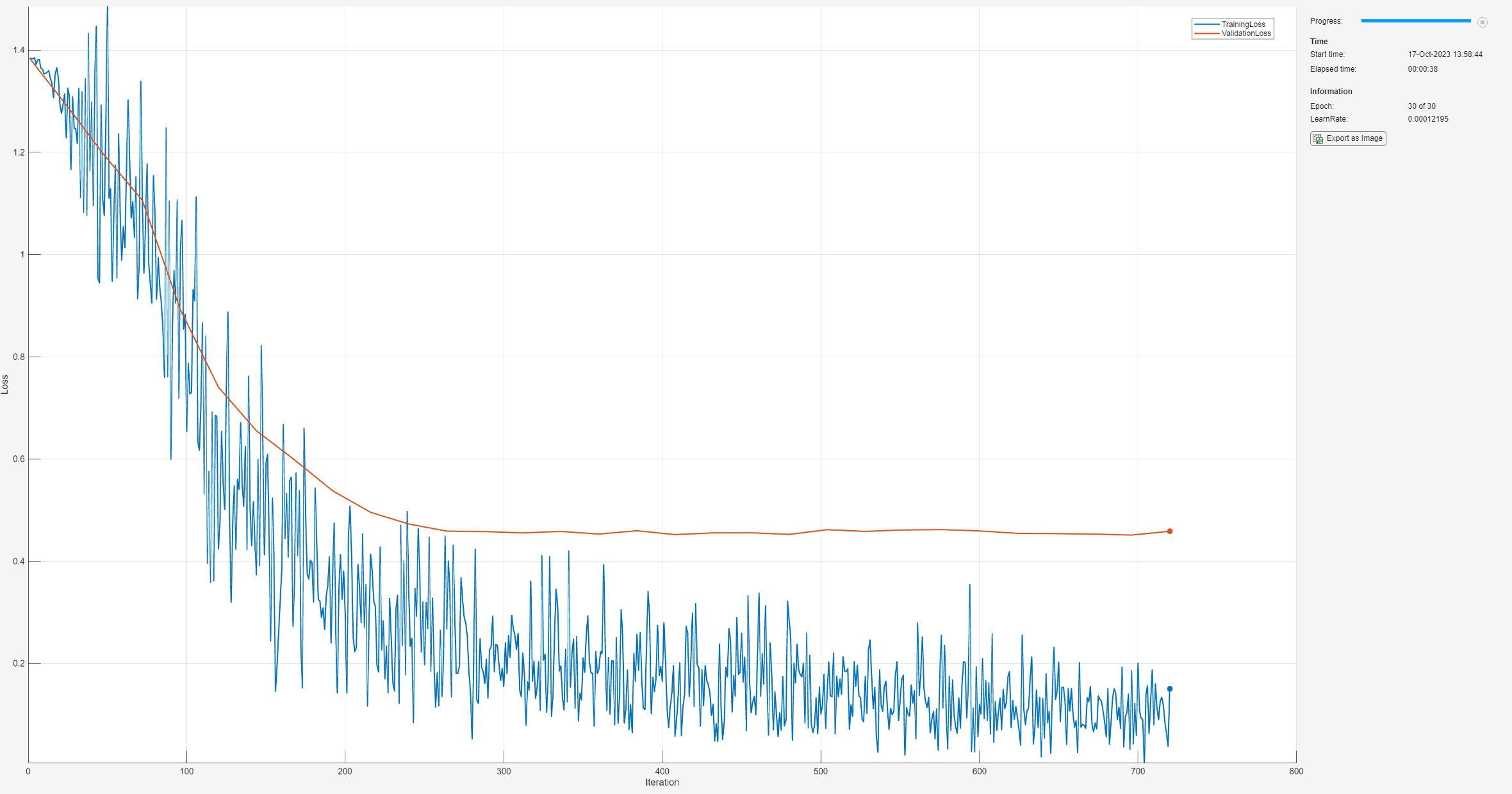
Initialize the TrainingProgressMonitor object. Because the timer starts when you create the monitor object, make sure that you create the object close to the training loop.
monitor = trainingProgressMonitor( ...
    Metrics=["TrainingLoss","ValidationLoss"], ...
    Info="Epoch", ...
    XLabel="Iteration");

groupSubPlot(monitor,"Loss",["TrainingLoss" "ValidationLoss"])
Train the network. For each epoch, shuffle the data and loop over mini-batches of data. At the end of each iteration, display the training progress. At the end of each epoch, validate the network using the validation data.
For each mini-batch:
Convert the documents to sequences of integers and one-hot encode the labels.
Evaluate the model loss and gradients using
dlfevaland themodelLossfunction.Update the network parameters using the custom update function and the
dlupdatefunction.Update the training plot.
Stop if the
Stopproperty of the monitor istrue. TheStopproperty value of theTrainingProgressMonitorobject changes totruewhen you click the Stop button.
epoch = 0;
iteration = 0;

% Loop over epochs.
while epoch < numEpochs && ~monitor.Stop
    epoch = epoch + 1;

    % Shuffle data.
    shuffle(mbq);

    % Loop over mini-batches.
    while hasdata(mbq) && ~monitor.Stop
        iteration = iteration + 1;

        % Read mini-batch of data.
        [X,T] = next(mbq);

        % Evaluate the model loss and gradients using dlfeval and the
        % modelLoss function.
        [loss,gradients] = dlfeval(@modelLoss,net,X,T);

        % Update the network parameters using SGD.
        updateFcn = @(parameters,gradients) sgdStep(parameters,gradients,learnRate);
        net = dlupdate(updateFcn,net,gradients);

        % Display the training progress.
        recordMetrics(monitor,iteration,TrainingLoss=loss);
        updateInfo(monitor,Epoch=(epoch+" of "+numEpochs));

        % Validate network.
        if iteration == 1 || ~hasdata(mbq)
            lossValidation = testnet(net,mbqValidation,"crossentropy");

            % Update plot.
            recordMetrics(monitor,iteration,ValidationLoss=lossValidation);
        end

        monitor.Progress = 100*iteration/numIterations;
    end
end
Test Model
Test the neural network using the testnet function. For single-label classification, evaluate the accuracy. The accuracy is the percentage of correct predictions. By default, the testnet function uses a GPU if one is available. Otherwise, the function uses the CPU. To select the execution environment manually, use the ExecutionEnvironment argument of the testnet function.
accuracy = testnet(net,mbqValidation,"accuracy")accuracy = 92.7083
Predict Using New Data
Classify the event type of three new reports. Create a string array containing the new reports.
reportsNew = [
    "Coolant is pooling underneath sorter."
    "Sorter blows fuses at start up."
    "There are some very loud rattling sounds coming from the assembler."];
Preprocess the text data using the preprocessing steps as the training documents.
documentsNew = preprocessText(reportsNew);
dsNew = arrayDatastore(documentsNew,OutputType="cell");
Create a minibatchqueue object that processes and manages the mini-batches of data. For each mini-batch:
Use the custom mini-batch preprocessing function
preprocessMiniBatchPredictors(defined at the end of this example) to convert documents to sequences. This preprocessing function does not require label data. To pass the word encoding to the mini-batch, create an anonymous function that takes one input only.Format the predictors with the dimension labels
"BTC"(batch, time, channel). Theminibatchqueueobject, by default, converts the data todlarrayobjects with underlying typesingle.To make predictions for all observations, return any partial mini-batches.
mbqNew = minibatchqueue(dsNew, ...
    MiniBatchSize=miniBatchSize, ...
    MiniBatchFcn=@(X) preprocessMiniBatchPredictors(X,enc), ...
    MiniBatchFormat="BTC", ...
    PartialMiniBatch="return");
Make predictions using the minibatchpredict function, and convert the classification scores to labels using the scores2label function. By default, the minibatchpredict function uses a GPU if one is available. Otherwise, the function uses the CPU. To select the execution environment manually, use the ExecutionEnvironment argument of the minibatchpredict function.
scores = minibatchpredict(net,mbqNew);
YNew = scores2label(scores,classes)'
YNew = 3×1 categorical array
    "Leak"
    "Electronic Failure"
    "Mechanical Failure"
Supporting Functions
Text Preprocessing Function
The function preprocessText performs these steps:
Tokenize the text using
tokenizedDocument.Convert the text to lowercase using
lower.Erase the punctuation using
erasePunctuation.
function documents = preprocessText(textData)

% Tokenize the text.
documents = tokenizedDocument(textData);

% Convert to lowercase.
documents = lower(documents);

% Erase punctuation.
documents = erasePunctuation(documents);

end
Mini-Batch Preprocessing Function
The preprocessMiniBatch function converts a mini-batch of documents to sequences of integers and one-hot encodes label data.
function [X,T] = preprocessMiniBatch(dataX,dataT,enc)

% Preprocess predictors.
X = preprocessMiniBatchPredictors(dataX,enc);

% Extract labels from cell and concatenate.
T = cat(1,dataT{1:end});

% One-hot encode labels.
T = onehotencode(T,2);

% Transpose the encoded labels to match the network output.
T = T';

end
Mini-Batch Predictors Preprocessing Function
The preprocessMiniBatchPredictors function converts a mini-batch of documents to sequences of integers.
function X = preprocessMiniBatchPredictors(dataX,enc)

% Extract documents from cell and concatenate.
documents = cat(4,dataX{1:end});

% Convert documents to sequences of integers.
X = doc2sequence(enc,documents);
X = cat(1,X{:});

end
See Also
wordEmbeddingLayer (Text Analytics Toolbox) | tokenizedDocument (Text Analytics Toolbox) | lstmLayer | doc2sequence (Text Analytics Toolbox) | sequenceInputLayer | wordcloud (Text Analytics Toolbox) | dlfeval | dlgradient | dlarray
Topics
- Custom Loss Functions
- Custom Training Loops
- Custom Training Loop Model Loss Functions
- Classify Text Data Using Deep Learning
- Create Simple Text Model for Classification (Text Analytics Toolbox)
- Analyze Text Data Using Topic Models (Text Analytics Toolbox)
- Analyze Text Data Using Multiword Phrases (Text Analytics Toolbox)
- Train a Sentiment Classifier (Text Analytics Toolbox)
- Sequence Classification Using Deep Learning
- Deep Learning in MATLAB