Frequency Response of a SISO System
This example shows how to plot the frequency response and obtain frequency response data for a single-input, single-output (SISO) dynamic system model.
Create a transfer function model and plot its frequency response.
H = tf([10,21],[1,1.4,26]);
bodeplot(H)
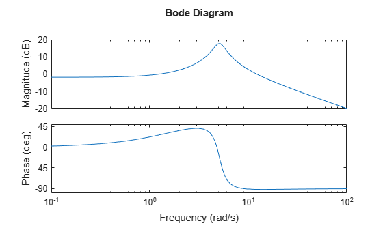
Unless you specify a frequency range to plot, bodeplot automatically chooses a frequency range based on the system dynamics.
Calculate the frequency response between 1 and 13 rad/s.
[mag,phase,w] = bode(H,{1,13});The bode command returns vectors mag and phase containing the magnitude and phase of the frequency response. The cell array input {1,13} tells bode to calculate the response at a grid of frequencies between 1 and 13 rad/s. bode returns the frequency points in the vector w.
See Also
bode | bodeplot | bodeoptions