Attitude Control in the HL-20 Autopilot - SISO Design

This example uses:

This is Part 3 of the example series on design and tuning of the flight control system for the HL-20 vehicle. This part shows how to tune a classic SISO architecture for controlling the roll, pitch, and yaw of the vehicle.

Background

This example uses the HL-20 model adapted from NASA HL-20 Lifting Body Airframe (Aerospace Blockset), see Part 1 of the series (Trimming and Linearization of the HL-20 Airframe) for details. The autopilot controlling the attitude of the aircraft consists of three inner loops and three outer loops.

In Part 2 (Angular Rate Control in the HL-20 Autopilot), we showed how to close the inner loops controlling the angular rates p,q,r. The following commands recap the corresponding steps. Note that this creates and configures an slTuner interface ST0 for interacting with the Simulink model.

load_system('csthl20_control')
CTYPE = 2;  % Select SISO architecture
HL20recapPart2

ST0

 
slTuner tuning interface for "csthl20_control":

No tuned blocks. Use the addBlock command to add new blocks.
9 Analysis points: 
--------------------------
Point 1: Signal "da;de;dr", located at 'Output Port 1' of csthl20_control/Flight Control System/Controller
Point 2: Signal "pqr", located at 'Output Port 2' of csthl20_control/HL20 Airframe
Point 3: 'Output Port 1' of csthl20_control/Flight Control System/Alpha_deg
Point 4: 'Output Port 1' of csthl20_control/Flight Control System/Beta_deg
Point 5: 'Output Port 1' of csthl20_control/Flight Control System/Phi_deg
Point 6: 'Output Port 1' of csthl20_control/Flight Control System/Controller/Classical/Demands
Point 7: Signal "p_demand", located at 'Output Port 1' of csthl20_control/Flight Control System/Controller/Classical/Roll-off1
Point 8: Signal "q_demand", located at 'Output Port 1' of csthl20_control/Flight Control System/Controller/Classical/Roll-off2
Point 9: Signal "r_demand", located at 'Output Port 1' of csthl20_control/Flight Control System/Controller/Classical/Roll-off3
 
No permanent openings. Use the addOpening command to add new permanent openings.
Properties with dot notation get/set access:
      Parameters         : [] 
      OperatingPoints    : [] (model initial condition will be used.)
      BlockSubstitutions : [3x1 struct]
      Options            : [1x1 linearize.SlTunerOptions]
      Ts                 : 0

Setup for Outer Loop Tuning

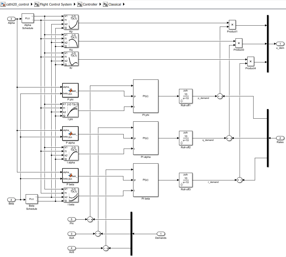
We now shift focus to the three gain-scheduled PI loops controlling roll (phi), angle of attack (alpha), and sideslip angle (beta). These loops could be tuned one at a time (3 loops and 40 operating points equals 120 design points). You could also use pidtune to tune the PI gains in batch mode for specific target bandwidth and phase margin requirements. Both approaches have caveats:

It is difficult to account for loop interactions.
The gains obtained at each design point may be inconsistent and require smoothing across operating points.

An alternative approach is the concept of "Gain Surface Tuning" [1] where you parameterize the gain schedules P(alpha,beta) and I(alpha,beta) as polynomial surfaces and use systune to tune the polynomial coefficients. This approach tackles all operating points at once and can account for loop interactions, in particular for stability margin considerations. This is the approach showcased here.

To tune the outer loops, we must close the inner loops and obtain a linearized model of the "plant" seen by the outer loops at each (alpha,beta) condition. We could ask slTuner to compute the corresponding transfer function, but this would effectively fix the inner-loop gains Kp,Kq,Kr to their values at the default operating condition. To get the correct linearization, we must tell slTuner that these gains vary with (alpha,beta). Block substitution is again the simplest way to do this. To mark Kp as varying, find the Product block used to multiply the error signal by Kp, and replace it by an array of gains, one for each (alpha,beta) condition.

ProductBlk = 'csthl20_control/Flight Control System/Controller/Classical/Product1';
BlockSub4 = struct('Name',ProductBlk,'Value',[0 ss(Kp)]);

It is easily verified that this block linearization amounts to multiplying the error signal by the varying quantity Kp computed above. Similarly, replace the corresponding Product blocks for Kq and Kr by varying gains.

ProductBlk = 'csthl20_control/Flight Control System/Controller/Classical/Product3';
BlockSub5 = struct('Name',ProductBlk,'Value',[0 ss(Kq)]);

ProductBlk = 'csthl20_control/Flight Control System/Controller/Classical/Product4';
BlockSub6 = struct('Name',ProductBlk,'Value',[0 ss(Kr)]);

ST0.BlockSubstitutions = [ST0.BlockSubstitutions ; BlockSub4 ; BlockSub5 ; BlockSub6];

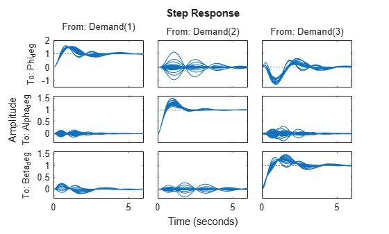
You can now plot the angular responses for the initial gain-schedule settings in the model.

T0 = getIOTransfer(ST0,'Demand',{'Phi_deg','Alpha_deg','Beta_deg'});
step(T0,6)

Tuning Goals

Basic control objectives include bandwidth (response time) and stability margins. Use the "MinLoopGain" and "MaxLoopGain" goals to set the gain crossover of the outer loops between 0.5 and 5 rad/s. Since all loop variables are expressed in degrees, no additional scaling is needed.

R1 = TuningGoal.MinLoopGain({'Phi_deg','Alpha_deg','Beta_deg'},0.5,1);
R1.LoopScaling = 'off';
R2 = TuningGoal.MaxLoopGain({'Phi_deg','Alpha_deg','Beta_deg'},tf(50,[1 10 0]));
R2.LoopScaling = 'off';

Use the "Margins" goal to impose adequate stability margins in each loop and across loops. This goal is based on the notion of disk margins which guarantees stability in the face of concurrent gain and phase variations in all three loops. Because the target margins of 7 dB and 40 degrees are difficult to obtain for extreme orientations (corners of the (alpha,beta) grid), we use a varying goal to relax the gain and phase margin requirements at the corners.

% Gain margins vs (alpha,beta)
GM = [...
   6     6     6     6     6
   6     6     7     6     6
   7     7     7     7     7
   7     7     7     7     7
   7     7     7     7     7
   7     7     7     7     7
   6     6     7     6     6
   6     6     6     6     6];

% Phase margins vs (alpha,beta)
PM = [...
   40         40          40         40        40
   40         40          45         40        40
   45         45          45         45        45
   45         45          45         45        45
   45         45          45         45        45
   45         45          45         45        45
   40         40          45         40        40
   40         40          40         40        40];

% Create varying goal
FH = @(gm,pm) TuningGoal.Margins('da;de;dr',gm,pm);
R3 = varyingGoal(FH,GM,PM);

Gain Schedule Tuning

To tune the P and I gain schedules for the outer loop, mark the three MATLAB Function blocks and three lookup table blocks as tunable.

TunedBlocks = {'P phi','P alpha','P beta','I phi','I alpha','I beta'};
ST0.addBlock(TunedBlocks)

Parameterize each tuned gain schedule as a polynomial surface in alpha and beta. Here we use quadratic surfaces for the proportional gains and multilinear surfaces for the integral gains.

% Grid of (alpha,beta) design points
alpha_vec = -10:5:25;	 % Alpha Range
beta_vec = -10:5:10;     % Beta Range
[alpha,beta] = ndgrid(alpha_vec,beta_vec);
SG = struct('alpha',alpha,'beta',beta);

% Proportional gains
alphabetaBasis = polyBasis('canonical',2,2);
P_PHI = tunableSurface('Pphi', 0.05, SG, alphabetaBasis);
P_ALPHA = tunableSurface('Palpha', 0.05, SG, alphabetaBasis);
P_BETA = tunableSurface('Pbeta', -0.05, SG, alphabetaBasis);
ST0.setBlockParam('P phi',P_PHI);
ST0.setBlockParam('P alpha',P_ALPHA);
ST0.setBlockParam('P beta',P_BETA);

% Integral gains
alphaBasis = @(alpha) alpha;
betaBasis = @(beta) abs(beta);
alphabetaBasis = ndBasis(alphaBasis,betaBasis);
I_PHI = tunableSurface('Iphi', 0.05, SG, alphabetaBasis);
I_ALPHA = tunableSurface('Ialpha', 0.05, SG, alphabetaBasis);
I_BETA = tunableSurface('Ibeta', -0.05, SG, alphabetaBasis);
ST0.setBlockParam('I phi',I_PHI);
ST0.setBlockParam('I alpha',I_ALPHA);
ST0.setBlockParam('I beta',I_BETA);

Note that we initialized each gain surface to a fixed value suggested by the baseline design. In general, it is not recommended to start from a zero or random initial point because the difficulty of the problem increases the likelihood of getting stuck in uninteresting local minima. Instead, a better strategy consists of tuning a fixed (non-scheduled) set of gains against the full set (or a relevant subset) of design points. Such "robust design" typically provides a good starting point for gain surface tuning.

You can now use systune to tune the 6 gain surfaces against the three tuning goals.

ST = systune(ST0,[R1 R2 R3]);

Final: Soft = 1.03, Hard = -Inf, Iterations = 40

The final objective value is close to 1 so the tuning goals are essentially met. Plot the closed-loop angular responses and compare with the baseline design.

T = getIOTransfer(ST,'Demand',{'Phi_deg','Alpha_deg','Beta_deg'});
step(T0,T,6)
legend('Baseline','Tuned','Location','SouthEast')

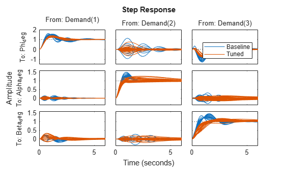
The results are comparable with the baseline with less oscillations in the roll and sideslip responses and a reduced amount of cross-coupling. Use viewSurf to inspect the tuned gain surfaces.

TV = getTunedValue(ST);
clf
% NOTE: setBlockValue updates each gain surface with the tuned coefficients in TV
subplot(3,2,1)
viewSurf(setBlockValue(P_PHI,TV))
subplot(3,2,3)
viewSurf(setBlockValue(P_ALPHA,TV))
subplot(3,2,5)
viewSurf(setBlockValue(P_BETA,TV))
subplot(3,2,2)
viewSurf(setBlockValue(I_PHI,TV))
subplot(3,2,4)
viewSurf(setBlockValue(I_ALPHA,TV))
subplot(3,2,6)
viewSurf(setBlockValue(I_BETA,TV))

Validation

To further validate this design, push the tuned gain surfaces to the Simulink model.

writeBlockValue(ST)

For the three lookup table blocks "I phi", "I alpha", "I beta", writeBlockValue samples the gain surfaces at the table breakpoints and updates the table data in the model workspace. For the MATLAB Function blocks "P phi", "P alpha", "P beta", writeBlockValue generates MATLAB code for the gain surface equations. For example, the code for the "P phi" block looks like

Simulink Coder automatically turns this MATLAB code into efficient embedded C code. Whether to use lookup tables or MATLAB Function blocks depends on the application. The MATLAB Function option ensures smooth variation of the gains as a function of alpha and beta (no kinks at breakpoints). It can also be more memory-efficient as it only needs to store the coefficients of the polynomial equation for the gain surface. On the other hand, evaluating the gain at a given (alpha,beta) point may take a few more operations than in a lookup table, and further adjustment of the gains is easier in a lookup table.

Once you pushed the gains to Simulink, the autopilot tuning is complete and you can simulate its behavior during the landing approach.

The performance is satisfactory but the linear responses showed a significant amount of cross-coupling between axes and we could not quite meet the stability margins target at the corner points of the (alpha,beta) range. Would it be beneficial to use a MIMO architecture that combines all three measurements of phi, alpha, beta to calculate the surface deflections? This idea is further explored in Part 4 of this series (Attitude Control in the HL-20 Autopilot - MIMO Design).

References

[1] P. Gahinet and P. Apkarian, "Automated tuning of gain-scheduled control systems," in Proc. IEEE Conf. Decision and Control, Dec 2013.