Main Content

metafeatures

Attractor metagene algorithm for feature engineering using mutual information-based learning

Description

example

M = metafeatures(X) returns the weighted sums of features M in X using the attractor metagene algorithm described in [1].

M is a r-by-n matrix. r is the number of metafeatures identified during each repetition of the algorithm. The default number of repetitions is 1. By default, only unique metafeatures are returned in M. If multiple repetitions result in the same metafeature, then just one copy is returned in M. n is the number of samples (patients or time points).

X is a p-by-n numeric matrix. p is the number of variables, features, or genes. In other words, rows of X correspond to variables, such as measurements of gene expression for different genes. Columns correspond to different samples, such as patients or time points.

[M,W] = metafeatures(X) returns a p-by-r matrix W containing metafeatures weights. M = W'*X. p is the number of variables. r is the number of unique metafeatures or the number of times the algorithm is repeated (the default is 1).

[M,W,GSorted] = metafeatures(X,G) uses a p-by-1 cell array of character vectors or string vector G containing the variable names and returns a p-by-r cell array of variable names GSorted sorted by the decreasing weight.

The ith column of GSorted lists the feature (variable) names in order of their contributions to the ith metafeature.

[M,W,GSorted,GSortedInd] = metafeatures(___) returns the indices GSortedInd such that GSorted = G(GSortedInd).

[___] = metafeatures(___,Name,Value) uses additional options specified by one or more Name,Value pair arguments.

[___] = metafeatures(T) uses a p-by-n table T. Gene names are the row names of the table. M = W'*T{:,:}.

[___] = metafeatures(T,Name,Value) uses additional options specified by one or more Name,Value pair arguments.

Note

It is possible that the number of metafeatures (r) returned in M can be fewer than the number of replicates (repetitions). Even though you may have set the number of replicates to a positive integer greater than 1, if each repetition returns the same metafeature, then r is 1, and M is 1-by-n. This is because, by default, the function returns only unique metafeatures. If you prefer to get all metafeatures, set 'ReturnUnique' to false. A metafeature is considered unique if the Pearson correlation between it and all previously found metafeatures is less than the 'UniqueTolerance' value (the default value is 0.98).

Examples

collapse all

Load the breast cancer gene expression data. The data was retrieved from the Cancer Genome Atlas (TCGA) on May 20, 2014 and contains gene expression data of 17814 genes for 590 different patients. The expression data is stored in the variable geneExpression. The gene names are stored in the variable geneNames.

load TCGA_Breast_Gene_Expression

The data has several NaN values.

sum(sum(isnan(geneExpression)))
ans =

        1695

Use the k-nearest neighbor imputation method to replace missing data with the corresponding value from an average of the k columns that are nearest.

geneExpression = knnimpute(geneExpression,3);

There are three common drivers of breast cancer: ERBB2, estrogen, and progestrone. metafeatures allows you to seed the starting weights to focus on the genes of interest. In this case, set the weight for each of these genes to 1 in three different rows of startValues. Each row corresponds to initial values for a different replicate (repetition).

erbb         = find(strcmp('ERBB2',geneNames));
estrogen     = find(strcmp('ESR1',geneNames));
progestrone  = find(strcmp('PGR',geneNames));

startValues = zeros(size(geneExpression,1),3);
startValues(erbb,1)        = 1;
startValues(estrogen,2)    = 1;
startValues(progestrone,3) = 1;

Apply the attractor metagene algorithm to the imputed data.

[meta, weights, genes_sorted] = metafeatures(geneExpression,geneNames,'start',startValues);

The variable meta has the value of three metagenes discovered for each sample. Plot these three metagenes to gain insight into the nature of gene regulation across different phenotypes of breast cancer.

plot3(meta(1,:),meta(2,:),meta(3,:),'o')
xlabel('ERBB2 metagene')
ylabel('Estrogen metagene')
zlabel('Progestrone metagene')

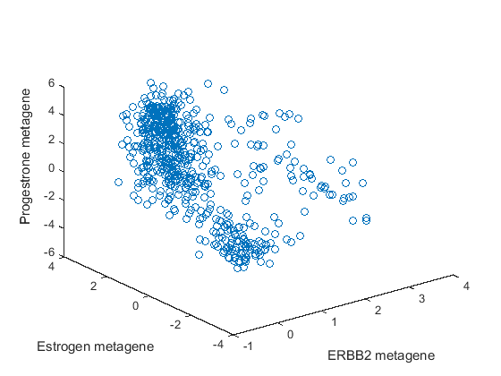
Based on the plot, observe the following.

  • There is a group of points clustered together with low values for all three metagenes. Based on mRNA levels, these could be triple-negative or basal type breast cancer.

  • There is a group of points that have high estrogen receptor metagene expression and span across both high and low progestrone metagene expression. There are no points with high progestrone metagene expression and low estrogen metagene expression. This is consistent with the observation that ER-/PR+ breast cancers are extremely rare [3].

  • The remaining points are the ERBB2 positive cancers. They have less representation in this data set than the hormone-driven and triple negative cancers.

Input Arguments

collapse all

Data, specified as a numeric matrix. Rows of X correspond to variables, such as measurements of gene expression. Columns correspond to different samples, such as patients or time points.

Variable names, specified as a cell array of character vectors or string vector.

Data, specified as a table. The row names of the table correspond to the names of features or genes, and the columns represent different samples, such as patients or time points.

Name-Value Arguments

Specify optional pairs of arguments as Name1=Value1,...,NameN=ValueN, where Name is the argument name and Value is the corresponding value. Name-value arguments must appear after other arguments, but the order of the pairs does not matter.

Before R2021a, use commas to separate each name and value, and enclose Name in quotes.

Example: 'Replicates',5 specifies to repeat the algorithm five times.

Tuning parameter for the number of metafeatures, specified as the comma-separated pair consisting of 'Alpha' and a positive number. This parameter controls the nonlinearity of the function that calculates the weights as described in the Attractor Metagene Algorithm. As alpha increases, the number of metafeatures tends to increase. This parameter is often the most important parameter to adjust in the analysis of a data set.

Example: 'Alpha',3

Option for choosing initial weights, specified as the comma-separated pair consisting of 'Start' and a character vector, string, or matrix. This table summarizes the available options.

OptionDescription
'random'Initialize the weights to a vector of positive weights chosen uniformly at random and scaled such that they sum to 1. Choose a different initial weight vector for each replicate. This option is the default.
'robust'If X or T has n columns, run the algorithm n times. On the ith evaluation of the algorithm, the weights are initialized to all zeros with the exception of the ith weight, which is set to 1. This option is useful when you are attempting to find all metafeatures of a data set.
matrixn-by-r matrix of initial weights. The algorithm runs r times. The weights in the ith run of the algorithm are initialized to the ith column of the matrix.

Example: 'Start','robust'

Number of times to repeat the algorithm, specified as the comma-separated pair consisting of 'Replicates' and a positive integer. This option is valid only with the 'random' start option. The default is 1.

Example: 'Replicates',2

Unique metafeatures flag, specified as the comma-separated pair consisting of 'ReturnUnique' and true or false. If true, then only the unique metafeatures are returned. The default is true.

This option is useful when the algorithm is repeated multiple times. By setting this option to true, you choose to look at just the unique metafeatures since the same set of metafeatures can be discovered for different initializations.

A metafeature is considered unique if the Pearson correlation between it and all previously found metafeatures is less than the 'UniqueTolerance' value (the default value is 0.98).

To run the algorithm multiple times, set the 'Replicates' name-value pair argument or the 'Start' option to 'robust' or a matrix with more than 1 row.

Example: 'ReturnUnique',false

Tolerance for metafeature uniqueness, specified as the comma-separated pair consisting of 'UniqueTolerance' and a real number between 0 and 1.

A metafeature is considered unique if the Pearson correlation between it and all previously found metafeatures is less than the 'UniqueTolerance' value.

Example: 'UniqueTolerance',0.90

Options for controlling the algorithm, specified as the comma-separated pair consisting of 'Options' and a structure. This table summarizes these options.

OptionDescription
DisplayLevel of output display. Choices are 'off' or 'iter'. The default is 'off'.
MaxIterMaximum number of iterations allowed. The default is 100.
ToleranceIf M changes by less than the tolerance in an iteration, then the algorithm stops. The default is 1e-6.
StreamsA RandStream object. If you do not specify any streams, metafeatures uses the default random stream.
UseParallelLogical value indicating whether to perform calculations in parallel if a parallel pool and Parallel Computing Toolbox™ are available. For problems with large data sets relative to the available system memory, running in parallel can degrade performance. The default is false.

Example: 'Options',struct('Display','iter')

Output Arguments

collapse all

Metafeatures, returned as a numeric matrix. It is an r-by-n matrix containing the weighted sums of the features in X. r is the number of replicates performed by the algorithm. n is the number of different samples such as time points or patients.

Note

It is possible that the number of metafeatures (r) returned in M can be fewer than the number of replicates (repetitions). Even though you may have set the number of replicates to a positive integer greater than 1, if each repetition returns the same metafeature, then r is 1, and M is 1-by-n. This is because, by default, the function returns only unique metafeatures. If you prefer to get all metafeatures, set 'ReturnUnique' to false. A metafeature is considered unique if the Pearson correlation between it and all previously found metafeatures is less than the 'UniqueTolerance' value (the default value is 0.98).

Metafeatures weights, returned as a numeric matrix. It is a p-by-r matrix. p is the number of variables. r is the number of replicates performed by the algorithm.

Sorted variable names, returned as a cell array of character vectors. It is a p-by-r cell array. The names are sorted by decreasing weight. The ith column of the GSorted lists the variable names in order of their contributions to ith metafeature.

If GSorted is requested without G or if T.Properties.RowNames is empty, then the algorithm names each variable (feature) as Vari, which corresponds to the ith row of X.

Index to GSorted, returned as a matrix of indices. It is a p-by-r matrix. The indices satisfy GSorted = G(GSortedInd) or GSorted = T.Properties.RowNames(GSortedInd).

More About

collapse all

Attractor Metagene Algorithm

The attractor metagene algorithm [1] is an iterative algorithm that converges to metagenes with important features. A metagene is defined as any weighted sum of gene expression using a nonlinear distance metric. The distance metric is a nonlinear variant of mutual information using binning and splines as described in [2]. In fact, the use of mutual information as a distance metric is one of major benefits of this algorithm since mutual information is a robust information theoretic approach to determine the statistical dependence between variables. Therefore, it is useful for analyzing relationships among gene expression. Another advantage is that the results of the algorithm tend to be more clearly linked with a phenotype defined by gene expression.

The algorithm is initialized by either random or user-specified weights and proceeds in these steps.

  1. The estimate of a metagene during the ith iteration of the algorithm is Mi=Wi*G, where Wi is a vector of weights of size 1-by-p (number of genes), and G is the gene expression matrix of size p-by-n (number of samples).

  2. Update the weights by Wj,i+1=J(Mi,Gj), where Wj,i+1 is the jth element of Wi+1, Gj is the jth row of G, and J is a similarity metric, which is defined as follows.

    • If the Pearson correlation between Mi and Gj is greater than 0, then J(Mi,Gj)=I(Mi,Gj)α, where I(Mi,Gj) is the measure of mutual information between two genes with minimum value 0 and maximum value 1, and α is any nonnegative number.

    • If the correlation is less than or equal to 0, then J(Mi,Gj)=0.

The algorithm iterates until the change in Wi between iterations is less than the defined tolerance, that is, WiWi1<tolerance or the maximum number of iterations is reached.

The Role of α

In the similarity metric of the algorithm, the parameter α controls the degree of nonlinearity. As α increases, the number of metagenes tends to increase. If α is sufficiently large, then each gene approximately becomes an attractor metagene. If α is zero, then all weights remain equal to each other. Therefore, there is only one attractor metagene representing the average of all genes.

Therefore, adjusting α for the data set under consideration is a key step in fine tuning the algorithm. In the case of [1], using the TCGA data from several types of cancer to identify attractor metagenes, α value of 5 resulted in between 50 and 150 attractor metagenes discovered from the data.

References

[1] Cheng, W-Y., Ou Yang, T-H., and Anastassiou, D. (2013). Biomolecular events in cancer revealed by attractor metagenes. PLoS Computational Biology 9(2): e1002920.

[2] Daub, C., Steuer, R., Selbig, J., and Kloska, S. (2004). Estimating mutual information using B-spline functions – an improved similarity measure for analysing gene expression data. BMC Bioinformatics 5, 118.

[3] Hefti, M.M., Hu, R., Knoblauch, N.W., Collins, L.C., Haibe-Kains, B., Tamimi, R.M., and Beck, A.H. (2013). Estrogen receptor negative/progesterone receptor positive breast cancer is not a reproducible subtype. Breast Cancer Research. 15:R68.

Extended Capabilities

Version History

Introduced in R2014b