Conventional Vehicle Spark-Ignition Engine Fuel Economy and Emissions
This example shows how to calculate the city and highway fuel economy and the emissions for a conventional vehicle with a 1.5-L spark-ignition (SI) engine. To run this example, make sure you have the city (FTP75) and the highway (HWFET) drive cycles installed. After you open the conventional vehicle reference application, in the Scenarios > Reference Generator subsystem, open the Drive Cycle Source block. Click Install additional drive cycles. For more information, see Install Drive Cycle Data.
setupconvehMPG;

Prepare the Conventional Vehicle Reference Application for Simulation
Name the Drive Cycle Source block and Visualization subsystem.
model = 'ConfiguredConventionalVirtualVehicle';
dcs = [model, '/Scenarios/Reference Generator/Drive Cycle/Drive Cycle Source'];
vis_sys = [model, '/Visualization'];
In the Visualization subsystem, log the emissions signal data.
pt_set_logging([vis_sys, '/Performance Calculations'], 'US MPG', 'Fuel Economy [mpg]', 'both');
pt_set_logging([vis_sys, '/Emission Calculations'], 'TP HC Mass (g/mi)', 'HC [g/mi]', 'both');
pt_set_logging([vis_sys, '/Emission Calculations'], 'TP CO Mass (g/mi)', 'CO [g/mi]', 'both');
pt_set_logging([vis_sys, '/Emission Calculations'], 'TP NOx Mass (g/mi)', 'NOx [g/mi]', 'both');
pt_set_logging([vis_sys, '/Emission Calculations'], 'TP CO2 Mass (g/km)', 'CO2 [g/km]', 'both');
Run City Drive Cycle Simulation
Configure the Drive Cycle Source block to run the city drive cycle (FTP75).
set_param(dcs,'cycleVar','FTP75');
Run a simulation of the city drive cycle. Plot the results.
tfinal = get_param(dcs, 'tfinal');
tf = extractBefore(tfinal ,' ');
save_system(model);
simout1 = sim(model,'ReturnWorkspaceOutputs','on', 'StopTime', tf);

logsout1 = simout1.get('logsout');
FECity = logsout1.get('Fuel Economy [mpg]');
plot(FECity);
### Searching for referenced models in model 'ConfiguredConventionalVirtualVehicle'.
### Total of 7 models to build.
### Starting serial model build.
### Successfully updated the model reference simulation target for: NoBMS
### Successfully updated the model reference simulation target for: NoDifferentialControl
### Successfully updated the model reference simulation target for: NoThermalControl
### Successfully updated the model reference simulation target for: NoVCU
### Successfully updated the model reference simulation target for: OpenLoopBraking
### Successfully updated the model reference simulation target for: SiEngineController
### Successfully updated the model reference simulation target for: TransmissionController

Build Summary

Model reference simulation targets:

Model                   Build Reason                                               Status                        Build Duration
===============================================================================================================================
NoBMS                   Target (NoBMS_msf.mexw64) did not exist.                   Code generated and compiled.  0h 0m 54.116s
NoDifferentialControl   Target (NoDifferentialControl_msf.mexw64) did not exist.   Code generated and compiled.  0h 0m 21.781s
NoThermalControl        Target (NoThermalControl_msf.mexw64) did not exist.        Code generated and compiled.  0h 0m 19.354s
NoVCU                   Target (NoVCU_msf.mexw64) did not exist.                   Code generated and compiled.  0h 0m 19.696s
OpenLoopBraking         Target (OpenLoopBraking_msf.mexw64) did not exist.         Code generated and compiled.  0h 0m 19.341s
SiEngineController      Target (SiEngineController_msf.mexw64) did not exist.      Code generated and compiled.  0h 0m 39.373s
TransmissionController  Target (TransmissionController_msf.mexw64) did not exist.  Code generated and compiled.  0h 0m 21.816s

7 of 7 models built (0 models already up to date)
Build duration: 0h 3m 34.564s
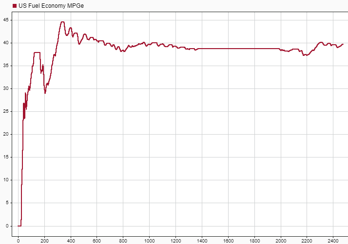
The results indicate that the fuel economy is approximately 38 mpg at the end of the drive cycle.
Run Highway Drive Cycle Simulation
Configure the Drive Cycle Source block to run the highway drive cycle (HWFET). Make sure that you have installed the highway drive cycle.
set_param(dcs,'cycleVar','HWFET');
Run a simulation of the highway drive cycle. Plot the results.
tfinal = get_param(dcs, 'tfinal');
tf = extractBefore(tfinal ,' ');
save_system(model);
simout2 = sim(model,'ReturnWorkspaceOutputs','on', 'StopTime', tf);

logsout2 = simout2.get('logsout');
FEHwy = logsout2.get('Fuel Economy [mpg]');
plot(FEHwy);
### Searching for referenced models in model 'ConfiguredConventionalVirtualVehicle'.
### Total of 7 models to build.
### Model reference simulation target for NoBMS is up to date.
### Model reference simulation target for NoDifferentialControl is up to date.
### Model reference simulation target for NoThermalControl is up to date.
### Model reference simulation target for NoVCU is up to date.
### Model reference simulation target for OpenLoopBraking is up to date.
### Model reference simulation target for SiEngineController is up to date.
### Model reference simulation target for TransmissionController is up to date.

Build Summary

0 of 7 models built (7 models already up to date)
Build duration: 0h 0m 3.1684s

The results indicate that the fuel economy is approximately 54 mpg at the end of the highway drive cycle.
Extract Results
Extract the final city and highway fuel economy results for the city and highway drive cycles from the logged data.
logsout1 = simout1.get('logsout');
FuelEconomyCity = logsout1.get('Fuel Economy [mpg]').Values.Data(end);
logsout2 = simout2.get('logsout');
FuelEconomyHwy = logsout2.get('Fuel Economy [mpg]').Values.Data(end);
Use the city and highway fuel economy results to compute the combined sticker mpg.
FECombined = 0.55*FuelEconomyCity + 0.45*FuelEconomyHwy;
Extract the tailpipe emissions from the city drive cycle.
HC = logsout1.get('HC [g/mi]').Values.Data(end);
CO = logsout1.get('CO [g/mi]').Values.Data(end);
NOx = logsout1.get('NOx [g/mi]').Values.Data(end);
CO2 = logsout1.get('CO2 [g/km]').Values.Data(end);
Display the fuel economy and city drive cycle tailpipe emissions results in the command window.
fprintf('\n***********************\n')
fprintf('FUEL ECONOMY\n');
fprintf('   City:     %4.2f mpg\n', FuelEconomyCity);
fprintf('   Highway:  %4.2f mpg\n', FuelEconomyHwy);
fprintf('   Combined: %4.2f mpg\n', FECombined);
fprintf('\nTAILPIPE EMISSIONS\n');
fprintf('   HC:   %4.3f [g/mi]\n',HC);
fprintf('   CO:   %4.3f [g/mi]\n',CO);
fprintf('   NOx:  %4.3f [g/mi]\n',NOx);
fprintf('   CO2:  %4.1f [g/km]\n',CO2);
fprintf('   NMOG: %4.3f [g/mi]',HC+NOx);
fprintf('\n***********************\n');
***********************
FUEL ECONOMY
   City:     39.70 mpg
   Highway:  54.26 mpg
   Combined: 46.25 mpg

TAILPIPE EMISSIONS
   HC:   0.001 [g/mi]
   CO:   0.000 [g/mi]
   NOx:  0.001 [g/mi]
   CO2:  138.3 [g/km]
   NMOG: 0.002 [g/mi]
***********************