Analyze Thermal Management System Effect on EV Range

R2026b

This example shows how thermal management system efficiency affects electric vehicle driving range. The coefficient of performance (COP) measures how much heating or cooling a thermal system delivers per watt of electricity it draws from the battery. Higher COP means less energy spent on climate control and more available for driving. In this example, you use a COP-based Virtual Vehicle Composer model to sweep COP, ambient temperature, and temperature setpoints to build a design map of estimated range and identify where improving system efficiency or tuning setpoints yields the most benefit. You can easily parameterize the COP-based vehicle model for early-stage tradeoff analysis, real-time simulation, and hardware-in-the-loop (HIL) environments.

To evaluate the thermal controller and extract the system-level COP used in the overlay, see Evaluate Electric Vehicle Thermal Controller Performance.

Build Electric Virtual Vehicle Model

Build your virtual vehicle using the Virtual Vehicle Composer app with these settings:

• Powertrain architecture — Electric Vehicle 1EM

• Vehicle Dynamics — Longitudinal Dynamics

• Model template — Simulink

• Thermal System — Managed Thermal System

The model includes a mapped battery, electric machines, longitudinal vehicle dynamics, and a COP-based thermal management subsystem.

currDir = pwd;
addpath(currDir);

mdl = "ConfiguredVirtualVehicleModel";
open_system(mdl)

Sweep COP and Ambient Temperature

Sweep COP from 1.5 to 5 and ambient temperature from -10 to 35 deg C to cover the full range from cold weather to mild conditions. Use parsim to run all combinations in parallel. The parsim function requires Parallel Computing Toolbox™ for parallel execution and falls back to serial execution if the toolbox is not available.

copSweepValues = [1.5 2 2.5 3 3.5 4 5];
ambientTempValues_K = [263.15 273.15 283.15 293.15 303.15 308.15];
[copGrid, tempGrid] = ndgrid(copSweepValues, ambientTempValues_K);
numCases = numel(copGrid);
dd = Simulink.data.dictionary.open("VirtualVehicleTemplate.sldd");
designData = getSection(dd, "Design Data");

Override signal logging to record only the two signals needed for range calculation (BattSoc and xdot). This reduces per-simulation output size and data transfer overhead.

loggingOverride = Simulink.SimulationData.ModelLoggingInfo.createFromModel(mdl);
busSelPath = "ConfiguredVirtualVehicleModel/Visualization/DataLogging/Bus Selector";
for k = 1:numel(loggingOverride.Signals)
    bp = loggingOverride.Signals(k).BlockPath;
    port = loggingOverride.Signals(k).OutputPortIndex;
    keepSignal = strcmp(bp.getBlock(1), busSelPath) && ismember(port, [1 4]);
    if ~keepSignal
        loggingOverride.Signals(k).LoggingInfo.DataLogging = false;
    end
end

Disable state and output saving to reduce computation during simulation. Use fast restart to compile the model once and reuse the compiled state across all parameter combinations.

simIn(1:numCases) = Simulink.SimulationInput(mdl);
for idx = 1:numCases
    simIn(idx) = simIn(idx).setVariable("PlntThrCOPe", copGrid(idx), Workspace=mdl);
    simIn(idx) = simIn(idx).setVariable("EnvAirTemp", tempGrid(idx), Workspace=mdl);
    simIn(idx) = simIn(idx).setModelParameter(SaveOutput="off", SaveState="off", SaveTime="off");
    simIn(idx) = simIn(idx).setModelParameter(DataLoggingOverride=loggingOverride);
end

simOut = parsim(simIn, ShowProgress="on", UseFastRestart="on");

Extract Estimated Range

Each simulation runs a single drive cycle. To estimate full-charge range, calculate how far the vehicle travels and how much state of charge (SOC) it uses in that cycle. Then, scale proportionally to find the total distance before SOC reaches 10%.

The code integrates vehicle speed to get cycle distance and measures the SOC drop over the cycle, and then, calculates:

$$

$\text{range}=\frac{\text{cycleDistance}\times ({\text{SOC}}_{\text{init}}-10)}{{\text{SOC}}_{used}}$

$$

socMin = 10;
estimatedRange_km = zeros(size(copGrid));
for idx = 1:numCases
    logData = simOut(idx).logsout;
    soc = logData.getElement("<BattSoc>");
    socInit = soc.Values.Data(1);
    socEnd = soc.Values.Data(end);
    vel = logData.getElement("<xdot>");
    xDisp = cumtrapz(vel.Values.Time, vel.Values.Data);
    cycleDistance_km = xDisp(end) / 1000;
    socUsed = socInit - socEnd;
    estimatedRange_km(idx) = cycleDistance_km * (socInit - socMin) / socUsed;
end

Analyze Range Sensitivity

The surface plot shows estimated range across the full COP and ambient temperature space. Steep regions indicate that COP improvement yields significant range gains. Flat regions indicate diminishing returns.

figure('Name','Range vs. COP and Ambient Temperature')
surf(copGrid, tempGrid - 273.15, estimatedRange_km)
xlabel("COP")
ylabel("Ambient Temperature (\circC)")
zlabel("Estimated Range (km)")
title("Driving Range vs. COP and Ambient Temperature")
colorbar

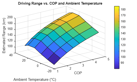
For each ambient temperature, compute how many additional km of range you gain per unit increase in COP. This value is the slope of range versus COP. At low COP (cold weather), the slope is steep, indicating that improving COP yields significant range gains. Above a COP value of 4, the slope flattens regardless of ambient condition, indicating diminishing returns.

ambientTemps_C = ambientTempValues_K - 273.15;
marginalThreshold = 5;
copTarget = zeros(1, numel(ambientTempValues_K));
figure('Name','Range Sensitivity by Ambient Temperature')
hold on
for tempIdx = 1:numel(ambientTempValues_K)
    rangeSlice = estimatedRange_km(:, tempIdx);
    marginalRange = diff(rangeSlice) ./ diff(copSweepValues(:));
    copMidpoints = (copSweepValues(1:end-1) + copSweepValues(2:end)) / 2;
    plot(copMidpoints, marginalRange, "-o", LineWidth=1.5, ...
        DisplayName=sprintf("%g\\circC", ambientTemps_C(tempIdx)))
    targetIdx = find(marginalRange < marginalThreshold, 1, 'first');
    if isempty(targetIdx)
        copTarget(tempIdx) = copSweepValues(end);
    else
        copTarget(tempIdx) = copMidpoints(targetIdx);
    end
end
hold off
xlabel("COP (midpoint)")
ylabel("Marginal Range Gain (km per unit COP)")
title("Range Sensitivity: Diminishing Returns by Ambient Temperature")
legend(Location="best")
grid on

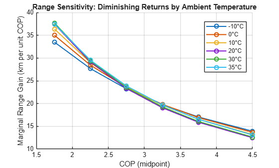
At each ambient temperature, find the COP value where adding one more unit of COP gives you less than 5 km of extra range. Beyond this point, investing in higher COP provides negligible benefit. This value becomes the COP target for the setpoint sweep.

copTargetTable = table(ambientTemps_C(:), copTarget(:), ...
    VariableNames=["AmbientTemp_C", "COP_Target"]);
disp(copTargetTable)

    AmbientTemp_C    COP_Target
    _____________    __________

         -10             5     
           0             5     
          10             5     
          20             5     
          30             5     
          35             5     

Sweep and Interpret Temperature Setpoints

With the COP target set, sweep battery and cabin temperature setpoints to see how much range is available from thermal tuning alone. Battery setpoints span 15 to 30 deg C, which is the realistic window for Li-ion cells. Cabin setpoints span 18 to 26 deg C. The sweep runs at three ambient conditions: cold, mild, and hot.

battSetpoints_C = [15 20 25 30];
cabinSetpoints_C = [18 21 24 26];
ambientSubset_C = [0 20 35];
ambientSubset_K = ambientSubset_C + 273.15;

battSetpoints_K = battSetpoints_C + 273.15;
cabinSetpoints_K = cabinSetpoints_C + 273.15;

copTargetSubset = interp1(ambientTemps_C, copTarget, ambientSubset_C, 'linear', 'extrap');

[ambGrid, battGrid, cabGrid] = ndgrid(1:numel(ambientSubset_K), 1:numel(battSetpoints_K), 1:numel(cabinSetpoints_K));
numSetpointCases = numel(ambGrid);

Configure each simulation case by mapping the flat loop index back to the 3D grid of ambient, battery setpoint, and cabin setpoint indices. Set COP to the target value for each ambient condition and apply the same performance settings as the first sweep.

simInSP(1:numSetpointCases) = Simulink.SimulationInput(mdl);
for idx = 1:numSetpointCases
    aIdx = ambGrid(idx);
    bIdx = battGrid(idx);
    cIdx = cabGrid(idx);
    simInSP(idx) = simInSP(idx).setVariable("PlntThrCOPe", copTargetSubset(aIdx), Workspace=mdl);
    simInSP(idx) = simInSP(idx).setVariable("EnvAirTemp", ambientSubset_K(aIdx), Workspace=mdl);
    simInSP(idx) = simInSP(idx).setVariable("CtrlThrBattTrgTemp", battSetpoints_K(bIdx), Workspace=mdl);
    simInSP(idx) = simInSP(idx).setVariable("CtrlThrCabTrgTemp", cabinSetpoints_K(cIdx), Workspace=mdl);
    simInSP(idx) = simInSP(idx).setModelParameter(SaveOutput="off", SaveState="off", SaveTime="off");
    simInSP(idx) = simInSP(idx).setModelParameter(DataLoggingOverride=loggingOverride);
end

simOutSP = parsim(simInSP, ShowProgress="on", UseFastRestart="on");

Extract estimated range from each simulation result and store it in a 3D array indexed by ambient condition, battery setpoint, and cabin setpoint.

rangeSetpoint_km = zeros(numel(ambientSubset_K), numel(battSetpoints_K), numel(cabinSetpoints_K));
for idx = 1:numSetpointCases
    aIdx = ambGrid(idx);
    bIdx = battGrid(idx);
    cIdx = cabGrid(idx);
    logData = simOutSP(idx).logsout;
    soc = logData.getElement("<BattSoc>");
    socInit = soc.Values.Data(1);
    socEnd = soc.Values.Data(end);
    vel = logData.getElement("<xdot>");
    xDisp = cumtrapz(vel.Values.Time, vel.Values.Data);
    cycleDistance_km = xDisp(end) / 1000;
    socUsed = socInit - socEnd;
    rangeSetpoint_km(aIdx, bIdx, cIdx) = cycleDistance_km * (socInit - socMin) / socUsed;
end

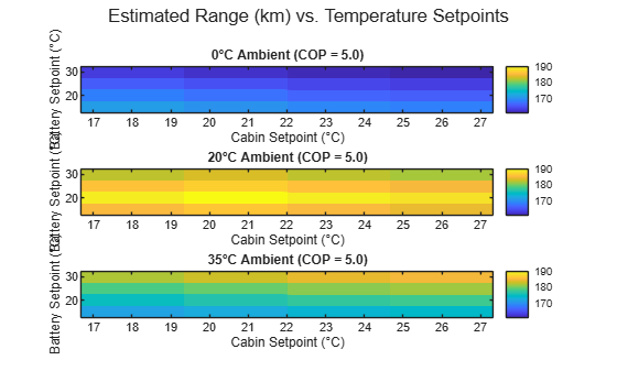
Display one heatmap per ambient condition. All three share the same color scale, so you can compare across conditions. The direction with more color gradient shows which setpoint has more influence.

Relaxing setpoints (warmer battery target, less cabin cooling) generally improves range but can increase thermal stress on components, or reduce occupant comfort.

figure('Name','Range vs. Setpoints by Ambient Condition')
for aIdx = 1:numel(ambientSubset_C)
    subplot(3, 1, aIdx)
    rangeSlice = squeeze(rangeSetpoint_km(aIdx, :, :));
    imagesc(cabinSetpoints_C, battSetpoints_C, rangeSlice)
    set(gca, 'YDir', 'normal')
    xlabel("Cabin Setpoint (\circC)")
    ylabel("Battery Setpoint (\circC)")
    title(sprintf("%g\\circC Ambient (COP = %.1f)", ambientSubset_C(aIdx), copTargetSubset(aIdx)))
    colorbar
    clim([min(rangeSetpoint_km(:)) max(rangeSetpoint_km(:))])
end
sgtitle("Estimated Range (km) vs. Temperature Setpoints")

Overlay Measured COP Values

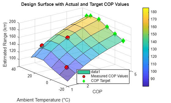
Load the COP lookup table that the Simscape thermal controller evaluation example produces. Instead of running additional simulations, interpolate range from the existing design surface. This process places each measured COP value on the surface to show where the actual system operates.

copData = load('cop_lookup_table.mat');
copLUT = copData.copLookupTable;

rangeOverlay_km = interp2(copSweepValues', ambientTemps_C', estimatedRange_km', ...
    copLUT.COPe(:), copLUT.ambientTemp_degC(:));

figure('Name','Design Surface with Measured COP Values')
surf(copGrid, tempGrid - 273.15, estimatedRange_km, FaceAlpha=0.6)
hold on
scatter3(copLUT.COPe(:), copLUT.ambientTemp_degC(:), rangeOverlay_km, ...
    100, 'r', 'filled', 'MarkerEdgeColor', 'k', DisplayName='Measured COP Values')
scatter3(copTarget, ambientTemps_C, interp2(copSweepValues', ambientTemps_C', estimatedRange_km', copTarget, ambientTemps_C), ...
    80, 'g', 'filled', 'Marker', 'd', DisplayName='COP Target')
hold off
xlabel("COP")
ylabel("Ambient Temperature (\circC)")
zlabel("Estimated Range (km)")
title("Design Surface with Actual and Target COP Values")
legend(Location="best")
colorbar

Next Steps

Based on where the measured COP values land on the design surface, choose whether to focus on improving system COP or optimizing temperature setpoints.

• Tune controller parameters — If measured COP sits on the steep portion of the surface, improving COP at those conditions yields meaningful range gains. Use the Simscape example to iterate on controller parameters and re-extract COP.

• Refine setpoints — If measured COP is near the target, focus on setpoint optimization. The sensitivity heatmaps show which combinations maximize range at each condition.

• Expand the sweep — Add more ambient temperatures, drive cycles, or payload conditions to build a comprehensive range map for the vehicle program.

• Deploy to hardware-in-the-loop (HIL) or software-in-the-loop (SIL) environment — Deploy the COP-based thermal model to an HIL or SIL environment for real-time controller testing.