Calculate Radiation Efficiency of Antenna

This example shows you how to calculate the radiation efficiency of an antenna or antenna array from the Antenna Toolbox™. The radiation efficiency of an antenna is defined as the ratio of the power radiated by an antenna to the power fed to the excitation port of the antenna. The power loss due to port impedance mismatch is not considered here.

The input power to the antenna can be written as

$$P_{in}=\frac{1}{2}{V}_{in}{I}_{in}^{*}.$$ (1)

Here, the input voltage and input current are represented by $$V_{in}$$ and $$I_{in}$$, respectively. $$I_{in}^{*}$$ is the complex conjugation of the input current. Calculate the power $$P_{rad}$$ radiated by the antenna by integrating the radiation intensity ($$U(\theta ,\varphi )$$) over the infinite radiation sphere ($$S_{\infty }$$)

$$P_{rad}={\int }_{S_{\infty }}U(\theta ,\varphi )sin\theta d\theta d\varphi .$$ (2)

The azimuth and elevation angles are denoted by $$\varphi$$ and $$\theta$$, respectively. The radiation efficiency ($${\eta }_r)$$ is defined as

$${\eta }_r=\frac{P_{rad}}{P_{in}}.$$ (3)

The difference between the input power and the radiated power is due to conduction loss in the metal-only antennas and due to both conduction loss and dielectric loss in the metal-dielectric antennas. The radiation efficiency is also alternately defined as the gain and directivity of the antenna. In other words,

$$G(\theta ,\varphi )={\eta }_{r}D(\theta ,\varphi ).$$ (4)

In an ideal lossless antenna, the radiation efficiency ($${\eta }_r$$) is 1.

Metal-Only Antenna

This example uses a Yagi-Uda antenna with the same dimensions as given in [1].

Create Geometry

Create the geometry of the Yagi-Uda antenna with two director elements of the length 131.9 mm and 126.5 mm, respectively. The spacing dimensions for the directors are 65.95 mm and 80.34 mm. The length of the exciter is 139.1 mm. The length and spacing values of the reflector are 141.5 mm and 88.13 mm, respectively. In [1], all the elements are thin wires with the radius of 0.6745 mm. However, this example uses the cylinder2strip function to model equivalent strips.

d=design(dipole,1e9);
radius=6.7450e-04; %Radius of thin wires
d.Width=cylinder2strip(radius); %Converting into equivalent stripwidth
d.Length=139.1e-03;
d.TiltAxis=[0 1 0];
d.Tilt=-90;
ant=design(yagiUda,1e9);
ant.Exciter=d;
ant.NumDirectors=2;
ant.DirectorLength=[131.9e-03;126.5e-03];
ant.DirectorSpacing=[65.95e-03;80.34e-03];
ant.ReflectorLength=141.5e-03;
ant.ReflectorSpacing=88.13e-03;

Visualize Antenna

Visualize the antenna, which is a default perfect electrical conductor (PEC) antenna with conductivity and thickness values of infinity and zero, respectively.

figure;
show(ant)

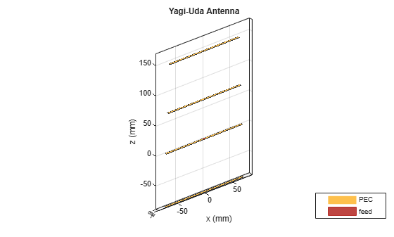
Using show function provides the name of the conductor and the feed location using different colors in the above figure.

Visualize Radiation Efficiency of PEC Antenna

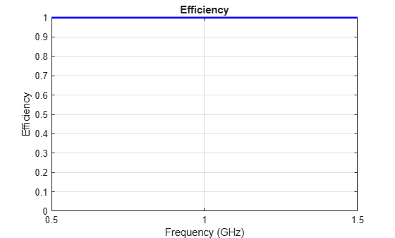
Plot the radiation efficiency of the PEC yagi-uda antenna using the efficiency function within the frequency range of 0.5-1.5 GHz with 31 sampling points. As the PEC antenna has no loss, it shows a radiation efficiency of 1 over the specified frequency range.

f=linspace(0.5e9, 1.5e9, 31);
efficiency(ant,f)

Visualize Directivity of PEC antenna

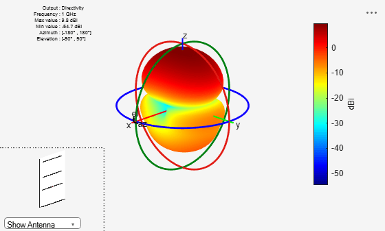
Calculate the directivity of the PEC Yagi-Uda antenna at a frequency of 1 GHz. Due to the absence of loss, the directivity and gain will be the same in the PEC antenna.

figure;
pattern(ant, 1e9)

Use Copper in Antenna Design

Set the conductor as copper from the metal catalog of the Antenna Toolbox. Modify the conductivity of the finite metal Yagi-Uda antenna using the properties of the metal object.

Use Copper Metal for Antenna Design

ant.Exciter.Conductor = metal('Copper');%Choose conductor from the metal catalog
ant.Exciter.Conductor.Conductivity = 1e5;%Same value used in the reference paper

Specify Metal Properties of Conductor

ant.Conductor = metal('Copper');%Choose the conductor from the metal catalog
ant.Conductor.Conductivity = 1e5;%same value used in the reference paper

Modify the conductivity and thickness of the finite metal Yagi-Uda antenna.

ant.Exciter.Conductor.Thickness = 700*1e-6;
ant.Conductor.Thickness = 700*1e-6;

Visualize Finite Metallic Antenna

Visualize the metallic Yagi-Uda antenna using the show function.

figure;
show(ant)

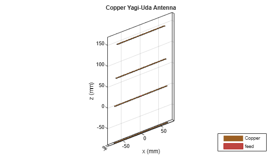
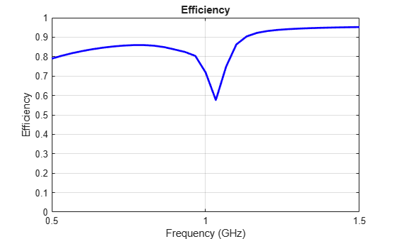
Plot Radiation Efficiency of Finite Metallic Antenna

Plot the radiation efficiency visualization of the metallic Yagi-Uda antenna at the frequency range of 0.5-1.5 GHz.

f = linspace(0.5e9, 1.5e9, 31);
figure;
efficiency(ant,f)

Plot Gain Pattern of Finite Metallic Antenna

Plot the gain pattern of the metallic Yagi-Uda antenna at a frequency of 1 GHz.

figure
pattern(ant,1e9)

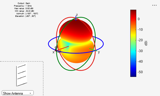
This shows that the gain of the antenna is reduced by 0.86 dB due to finite conduction loss. The efficiency value closely matches the analytical results in [1].

Metal-Dielectric Antenna

Create a microstrip patch antenna from [2]. The numerical analysis in [2] uses the finite-difference time-domain (FDTD) technique. However, this example uses the method of moments (MoM) solver from the Antenna Toolbox to analyze the antenna.

Create Geometry

Create the geometry of the microstrip patch antenna with a PEC conductor and lossy substrate of 1.57 mm thickness.

f = 1.59e9; %Solution frequency
lambda = 3e8/f;
d = dielectric('FR4'); %Selecting the substrate from the  dielectric catalog
d.EpsilonR = 4.36;
d.LossTangent = 2/100;%Indicates the lossy substrate
ant = patchMicrostrip('Substrate',d);
ant.Height = 1.57e-3;
ant.Substrate.Thickness = 1.57e-3;
ant.Length = 45e-3;
ant.Width = 45e-3;
ant.GroundPlaneLength = 20e-2;
ant.GroundPlaneWidth = 13.5e-2;
ant.FeedOffset = [20e-3 0];
ant.FeedWidth = lambda/200;

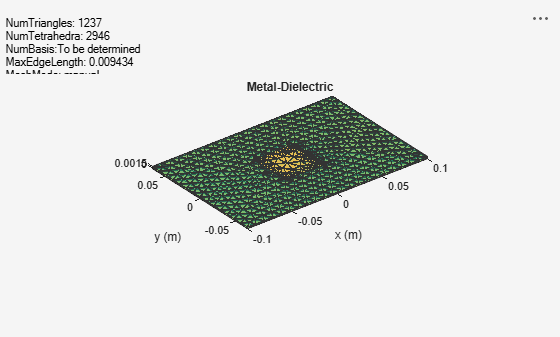
Manual Meshing of Microstrip Patch Antenna

Mesh the antenna by using the maximum edgelength of the RWG basis functions as lambda/20 where the free-space wavelength at the solution frequency of 1.5 GHz is lambda.

figure;
mesh(ant,'MaxEdgeLength',lambda/20)

Visualize Microstrip Patch Antenna

Visualize the antenna.

figure;
show(ant)

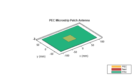
Calculate Radiation Efficiency of Microstrip Antenna with PEC Metal and Lossy Substrate

Calculate the radiation efficiency in absolute and logarithmic values. As the metal is PEC, the resultant loss is due to the lossy substrate.

E1 = efficiency(ant,f)

E1 = 
0.3045

E1_log = 10*log10(E1)

E1_log = 
-5.1638

Plot Directivity of Microstrip Antenna with PEC Metal and Lossy Substrate

Plot the directivity of the microstrip antenna using pattern function. The directivity does not depend on the conduction and dielectric losses.

figure
pattern(ant,f,'Type', 'Directivity')

Plot Gain of Microstrip Antenna with PEC Metal and Lossy Substrate

Plot the gain of the microstrip antenna with PEC metal and lossy substrate. The gain value is less than the directivity value due to the dielectric loss. The difference in the gain and directivity values matches closely with the log value of the radiation efficiency $$E{1}_{log}$$.

figure;
pattern(ant,f,'Type', 'Gain')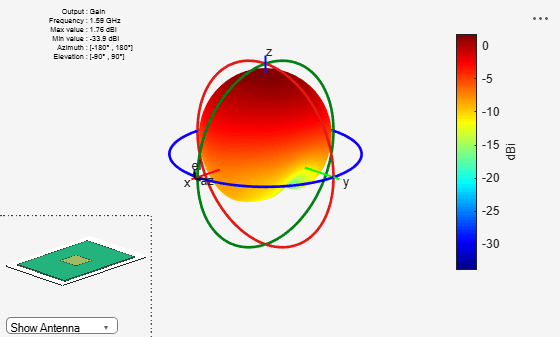

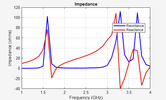
Impedance of Microstrip Antenna with PEC Metal and Lossy Substrate

Plot the impedance variation of the microstrip antenna with PEC metal and lossy substrate in the frequency range of 1-4 GHz.

f1 = linspace(1e9,4e9,31);
figure
impedance(ant,f1)

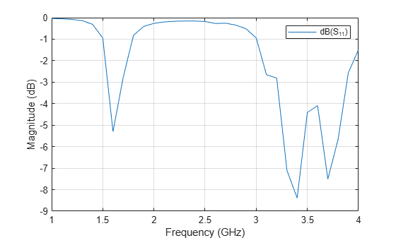
Return Loss of Microstrip Antenna with PEC Metal and Lossy Substrate

Plot the return loss variation of the microstrip antenna with PEC metal and lossy substrate.

figure;
s1 = sparameters(ant,f1,50);
rfplot(s1);

Change Conductor Properties of Microstrip Antenna

Set conductor of antenna as a lossy metal. Use metal object to change conductor to copper.

ant.Conductor = metal('Copper');

Visualize Microstrip Antenna with Lossy Metal and Lossy Substrate

Visualize of the microstrip antenna with a copper conductor and FR4 substrate.

figure;
show(ant)

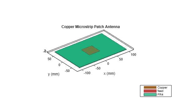
Calculate Radiation Efficiency of Microstrip Antenna with Lossy Metal and Lossy Substrate

Calculate the radiation efficiency in absolute and logarithmic values. The radiation efficiency is lower due to conduction loss in addition to the dielectric loss.

E2 = efficiency(ant,f)

E2 = 
0.2270

E2_log = 10*log10(E2)

E2_log = 
-6.4397

Plot Gain of Microstrip Antenna with Lossy Metal and Lossy Substrate

Plot the gain of the microstrip antenna with a copper conductor and FR4 substrate.

figure;
pattern(ant,f,'Type', 'Gain')

The gain value is less than the directivity value due to both the conduction loss and the dielectric losses. The difference in the gain and directivity matches closely with the log value of the radiation efficiency $$E{2}_{log}$$.

Conclusion

The radiation efficiencies computed using the Antenna Toolbox for both the metallic and metal-dielectric antennas are found to match closely as reported in the references that use different analytic [1] or numerical techniques [2].

References

[1] Shahpari, Morteza, and David V. Thiel. "Fundamental limitations for antenna radiation efficiency," IEEE Transactions on Antennas and Propagation, Vol. 66, No. 8, 2018.

[2] Ph. Leveque, A. Reineix and B. Jecko, “Modelling of Dielectric Losses in Microstrip Patch Antennas: Application of FDTD Method”, Electronics Letters, Vol. 28, No. 6, March 1992.