Design and Analyze Tapered-Slot SIW Filtenna
This example shows how to create the substrate-integrated-waveguide-based (SIW-based) antipodal filtenna described in [1] with a modified feeding network. A filtenna is a planar antenna with a built-in filter, which can be used to provide frequency agility for communicating at different frequencies without causing any interference to the adjacent bands.You can also use a filtenna to avoid undesired frequencies when you use it as a receiver.
The SIW filtenna design in this example has an operating range of 23.8 GHz to 40 GHz, maximum gain of 10.25 dB, and a maximum out-of-band suppression of 20.55 dB.
This figure shows the top view of the filtenna.

This figure shows the bottom view of the filtenna.
.
Create SIW Filtenna
Define the SIW patch, radiator, taper, feedline, ground plane, and slit dimensions as well as slit and via locations.
l_siw = 6.2e-3; % SIW patch length
l_arm = 25e-3; % Radiator length
l_taper = 3e-3; % Taper length
l_feed = 1.5e-3; % Feedline length
w_feed = 0.7826e-3; % Feedline width
w_taper = 1.745e-3; % Taper width
w_ant = 9.3e-3; % Antenna width
w_siw = 4.9e-3; % SIW patch width
w_arm = 5.55e-3; % Radiator and ground plane width
l_gnd = l_siw + l_taper + l_feed; % Ground plane length in the botto layer
w_gnd = w_ant; % Ground plane width
l_ant = l_feed + l_taper + l_siw + l_arm; % Total length of the antenna
viaX = -l_ant/2 + l_feed + l_taper + 0.25e-3; % Via start point location on x-axis
viaY = w_siw/2; % Via start point location on y-axis
p_siw = 0.7e-3; % Via pitch
l_slit = 0.45e-3; % Side slit length
w_slit = 1.6e-3; % Side slit width
slitX = -l_ant/2 + l_feed + l_taper + l_siw + l_slit/2; % X-coordinate of slit position
slitY = -w_ant/2 + w_slit/2; % Y-coordinate of slit position
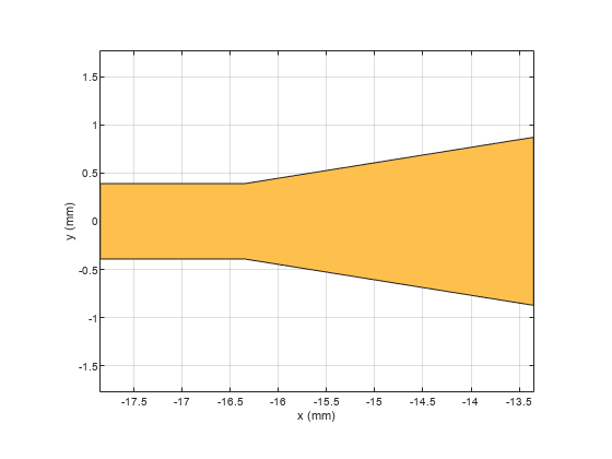
Create Tapered Microstrip Line
Use the specified dimesions to create a microstrip transmission line. Use a tapered section to match the impedance with a 50 Ω microstrip line in which the quasi-TEM and TE10 modes are dominant. Create a microstrip line up to the SIW transition trace. Visualize the transition using the show method.
feedline = antenna.Rectangle(Length=l_feed,Width=w_feed,Center=[-l_ant/2+l_feed/2 0]);
taper = antenna.Polygon;
taper.Name = "taper";
taper.Vertices = [-l_ant/2+l_feed w_feed/2;-l_ant/2+l_feed+l_taper w_taper/2;-l_ant/2+l_feed+l_taper -w_taper/2;-l_ant/2+l_feed -w_feed/2];
transition = taper + feedline;
figure(Name="Tapered Micostrip Line")
show(transition);
Create SIW
Use antenna.Rectangle object to create the SIW. This object adds high-pass filter characteristics to the lower bound of the antenna resonance. The SIW operates at a frequency of 25 GHz.
Create series of vias to the SIW transmission line.
siw = antenna.Rectangle(Length=l_siw, Width=w_ant, Center=[-l_ant/2+l_feed+l_taper+l_siw/2 0]);
for i=1:9
    viapointX(i) = viaX + (i-1)*(p_siw);
    viapointY(i) = -viaY;
    layer1(i) = 1;
    layer2(i) = 3;
    vialoc1 = [viapointX' viapointY' layer1' layer2'];
end
for i=1:9
    viapointX(i) = viaX + (i-1)*(p_siw);
    viapointY(i) = viaY;
    layer1(i) = 1;
    layer2(i) = 3;
    vialoc2 = [viapointX' viapointY' layer1' layer2'];
end
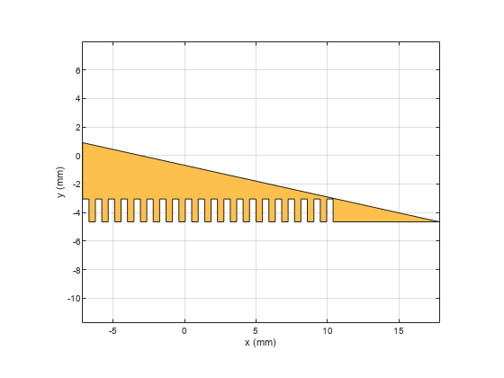
Create Radiator
Create the antipodal antenna with two arms named as topArm and bottomArm. Use antenna.Polygon and antenna.Rectangle functions to create the arms of antipodal antenna with slits. Visualize the arms using the show function.
Create the top radiating arm.
topArm = antenna.Polygon;
topArm.Vertices = [-l_ant/2+l_feed+l_taper+l_siw -w_ant/2;...
    -l_ant/2+l_feed+l_taper+l_siw -w_ant/2+w_arm;...
    -l_ant/2+l_feed+l_taper+l_siw+l_arm -w_ant/2];
for i = 1:20
Slit = antenna.Rectangle(Length=l_slit, Width=w_slit, Center=[slitX slitY]);
slitX = slitX + 2*l_slit;
topArm = topArm - Slit;
end
figure(Name="Top Arm")
show(topArm)
Create the top layer.
topLayer = siw + feedline + taper + topArm;
Ceate the bottom radiating arm.
bottomArm = copy(topArm);
bottomArm = mirrorX(bottomArm);
gnd = antenna.Rectangle(Length=l_gnd, Width=w_ant, Center=[-l_ant/2+l_gnd/2 0]);
Create the bottom layer.
Bottomlayer = gnd + bottomArm;
figure(Name="Bottom Arm")
show(bottomArm)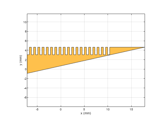
Create Printed Circuit Board (PCB) Antenna
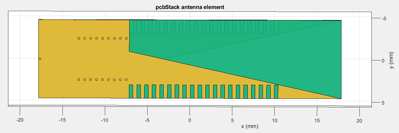
Use the pcbStack object to create a PCB antenna using the SIW filtenna geometry. You can extract the shape of the top layer by querying the Layers property.
Visualize the antenna using the show function.
siwFiltenna = pcbStack ;
substrate = dielectric("Teflon");
substrate.EpsilonR = 2.2;
substrate.Thickness = 0.254e-3;
siwFiltenna.BoardThickness = 0.254e-3;
siwFiltenna.Layers = {topLayer,substrate,Bottomlayer};
boardShape = antenna.Rectangle(Length=l_ant, Width=w_ant, Center=[0 0]);
siwFiltenna.BoardShape = boardShape;
siwFiltenna.FeedDiameter = w_feed/4;
siwFiltenna.FeedLocations = [-l_ant/2+w_feed/4 0 3 1];
siwFiltenna.ViaLocations = [vialoc1; vialoc2]
siwFiltenna =
pcbStack with properties:
Name: 'MyPCB'
Revision: 'v1.0'
BoardShape: [1x1 antenna.Rectangle]
BoardThickness: 2.5400e-04
Layers: {[1x1 antenna.Polygon] [1x1 dielectric] [1x1 antenna.Polygon]}
FeedLocations: [-0.0177 0 3 1]
FeedDiameter: 1.9565e-04
ViaLocations: [18x4 double]
ViaDiameter: []
FeedViaModel: 'strip'
FeedVoltage: 1
FeedPhase: 0
Conductor: [1x1 metal]
Tilt: 0
TiltAxis: [1 0 0]
Load: [1x1 lumpedElement]
siwFiltenna.ViaDiameter = 0.00025;
siwFiltenna.FeedViaModel = "square";
siwFiltenna.FeedVoltage = 1;
siwFiltenna.FeedPhase = 0;
show(siwFiltenna)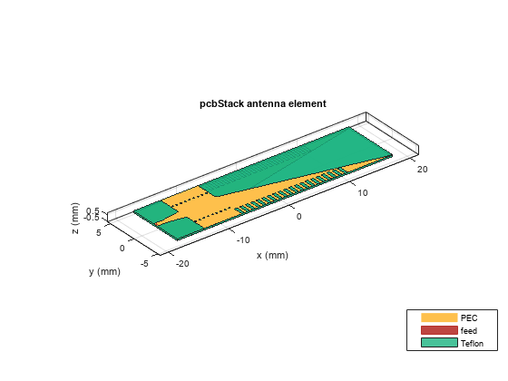
Analyze Filtenna
Use the mesh function to mesh the SIW filtenna. Set the maximum edge length to one eighth of the wavelength to get a fine mesh.
plotfrequency = 40*1e9;
lambda = 3e8/plotfrequency; % Wavelength
mesh(siwFiltenna, MaxEdgeLength=lambda/8, MinEdgeLength=lambda/14);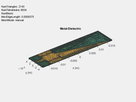
Estimate memory requirement
Use the memoryEstimate function to calculate the memory required to solve the structure.
memEst = memoryEstimate(siwFiltenna,25e9)
memEst =
'2.6 GB'
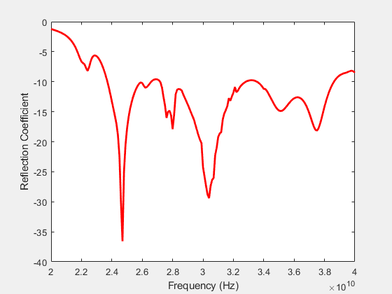
Calculate S-Parameters
To calculate and plot the S-parameters, set the plotSParams variable to true. Calculating and plotting the S-Parameters can take a long time. To save time, set plotSParams to false and use the precomputed results in the FilterAntennaData MAT file attached to this example for the analysis.
frequencyRange = (20:0.1:40)*1e9;
plotSParams = false;
if plotSParams
    s = sparameters(siwFiltenna,frequencyRange);
    rfplot(s)
end
Load the data from the FiltennaData MAT file, which contains the simulated and measured data in the S11_simulated, S11_measured, pattern_simulated, and pattern_measured variables. Use S11_simulated to plot the S-Parameters.
load FiltennaData.mat
plot(frequencyRange,S11_simulated,"r",LineWidth=2);
xlabel("Frequency (Hz)");
ylabel("Reflection Coefficient");
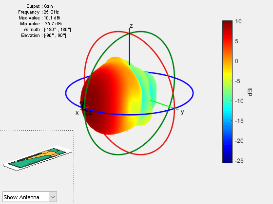
Plot Radiation Pattern
Use the pattern function to plot the 3-D radiation pattern at 25 GHz.
pattern(siwFiltenna,25e9);
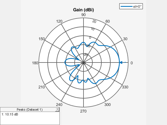
Use the pattern function to plot the 2-D radiation pattern at an elevation angle of 0 degrees.
pattern(siwFiltenna,25e9,0:1:360,0);
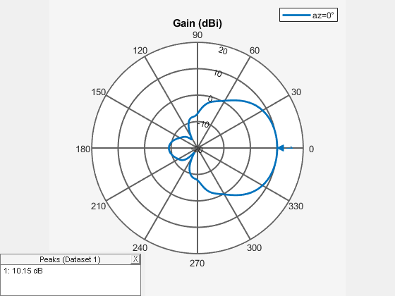
Use the pattern function to plot the 2-D radiation pattern at an azimuth angle of 0 degrees.
pattern(siwFiltenna,25e9,0,0:1:360);
Surface Current Distribution
Use the current function to plot the current distribution of the antenna at 25 GHz.
current(siwFiltenna,25e9, scale="log");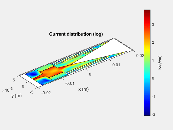
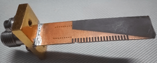
Compare Simulated and Measured Results
The SIW filtenna was built and tested for the reflection coefficient and the radiation pattern. The reflection coefficient was measured on a Keysight© N5224B PNA Network Analyzer. The radiation pattern measurements were performed in an anechoic chamber.
This figure shows the top view of the antenna.

This figure shows the bottom view of the antenna.
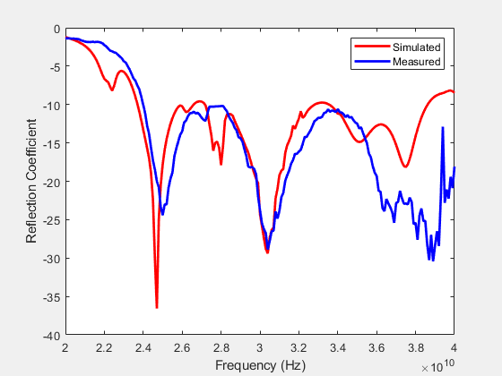
Compare the simulated and measured reflection coefficients as functions of frequency.
  plot(frequencyRange,S11_simulated,"r",LineWidth=2);
  hold on
  plot(frequencyRange,S11_measured',"b",LineWidth=2);
  hold off
  xlabel("Frequency (Hz)");
  ylabel("Reflection Coefficient");
  legend("Simulated","Measured");
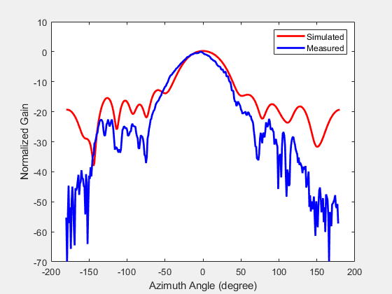
Compare the simulated and measured radiation patterns as functions of azimuth angles. The proposed antenna exhibits stable radiation characteristics with a gain of 10.25 dB at 25 GHz.
  plot(-180:1:180,pattern_simulated,"r",LineWidth=2);
  hold on
  plot(-180:1:180,pattern_measured',"b",LineWidth=2);
  hold off
  xlabel("Azimuth Angle (degree)");
  ylabel("Normalized Gain");
  legend("Simulated","Measured");
Conclusion
The designed antenna has a maximum gain of 10.25 dB and a bandwidth of 23.8 GHz to 40 GHz. You verify the efficiency of the filtenna by comparing the simulated value against a prototype that has been fabricated and measured. The measured and simulated results agree well. The filtenna is a promising candidate for compact 5G/B5G millimeter-wave communication system.
Reference
[1] Mengyun Hu, Zhiqiang Yu, Jun Xu, Ji Lan, Jianyi Zhou, and Wei Hong. "Diverse SRRs Loaded Millimeter-Wave SIW Antipodal Linearly Tapered Slot Filtenna With Improved Stopband," in IEEE Transactions on Antennas and Propagation, 69, no. 12, (December 2021): 8902–7. https://doi.org/10.1109/TAP.2021.3090854.
Select a Web Site
Choose a web site to get translated content where available and see local events and offers. Based on your location, we recommend that you select: United States.
You can also select a web site from the following list
Americas
- América Latina (Español)
- Canada (English)
- United States (English)
Europe
- Belgium (English)
- Denmark (English)
- Deutschland (Deutsch)
- España (Español)
- Finland (English)
- France (Français)
- Ireland (English)
- Italia (Italiano)
- Luxembourg (English)
- Netherlands (English)
- Norway (English)
- Österreich (Deutsch)
- Portugal (English)
- Sweden (English)
- Switzerland
- United Kingdom (English)
Asia Pacific
- Australia (English)
- India (English)
- New Zealand (English)
- 中国
- 日本Japanese (日本語)
- 한국Korean (한국어)