Artificial Intelligence (AI) for Rapid Analysis and Design of Patch Antenna
This example shows how to use artificial intelligence (AI) to rapidly analyze and design antennas from the Antenna Toolbox™ catalog.
Learn how the AIAntenna object can be used to take advantage of the speed of AI-based analysis without the need for prior machine learning experience. Follow this example to:
Create an antenna for AI-based analysis using
AIAntenna.Use AI to analyze a specific antenna design.
Rapidly explore antennas across the design space.
Create Antenna for AI-Based Analysis
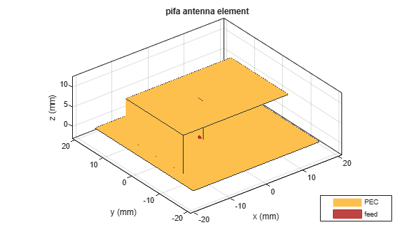
Using design with ForAI=true, create an AIAntenna for AI-based analysis of a planar inverted-F antenna (PIFA) designed to resonate around 2.4 GHz.
antType = pifa;
fd = 2.4e9;
pifaAI = design(antType,fd,ForAI=true);
Calculate the resonant frequency of the prototype antenna using AI-based analysis by calling resonantFrequency on the AIAntenna object, noting that the calculated resonant frequency is higher but approximately equal to the design frequency of 2.4 GHz.
resonantFrequencyAI0 = resonantFrequency(pifaAI)
resonantFrequencyAI0 =
2.4091e+09
Now calculate the bandwidth using AI-based analysis. The bandwidth function outputs the absolute bandwith, the lower and upper frequencies of the bandwidth, and whether the antenna is matched at 50 ohms. An antenna is matched when its S11 plot dips below -10 dB. Here, the antenna has a bandwidth, indicating it is matched because a frequency range exists where the S11 is less than -10 dB.
[bandwidthAI0,lowerFrequencyAI0,upperFrequencyAI0,matchingAI0] = bandwidth(pifaAI)
bandwidthAI0 =
1.4809e+08
lowerFrequencyAI0 =
2.3186e+09
upperFrequencyAI0 =
2.4667e+09
matchingAI0 = categorical
     Matched
Calculate Resonant Frequency and Bandwidth of Specific Antenna Design
To achieve a wider bandwidth [1], increase the width to be 0.7 times the length while keeping the short pin width equal to the width.
First, query the AIAntenna object. The tunable parameters of a PIFA for AI-based analysis are length, width, height, and short pin width.
pifaAI
pifaAI =
  AIAntenna with properties:

   Antenna Info
               AntennaType: 'pifa'
    InitialDesignFrequency: 2.4000e+09

   Tunable Parameters
                    Length: 0.0292
                     Width: 0.0194
                    Height: 0.0097
             ShortPinWidth: 0.0194

Show read-only properties
View the non-tunable properties by calling showReadOnlyProperties.
showReadOnlyProperties(pifaAI)
              SubstrateName: 'Air'
          SubstrateEpsilonR: 1
       SubstrateLossTangent: 0
         SubstrateThickness: 0.0097
    SubstrateFrequencyModel: 'Constant'

          GroundPlaneLength: 0.0350
           GroundPlaneWidth: 0.0350
          PatchCenterOffset: [0 0]
                 FeedOffset: [-0.0019 0]

              ConductorName: 'PEC'
      ConductorConductivity: Inf
         ConductorThickness: 0

                       Tilt: 0
                   TiltAxis: [1 0 0]

              LoadImpedance: []
              LoadFrequency: []
               LoadLocation: 'feed'
Define the desired design specifications.
W = pifaAI.Length*0.7;
shortPinW = W
shortPinW =
0.0204
Before modifying your prototype to meet the desired design, use tunableRanges to verify that your desired value is within the tunable ranges supported for AI-based analysis of your antenna. In this case, the desired width of 0.0204 m is within the tunable range of 0.0165 m and 0.0224 m. The same can be said of the short pin width.
tRanges = tunableRanges(pifaAI)
tRanges=2×4 table
                                Length                  Width                   Height               ShortPinWidth
                         ____________________    ____________________    _____________________    ____________________

                           min         max         min         max          min         max         min         max
                         ________    ________    ________    ________    _________    ________    ________    ________

    resonantFrequency    0.024792    0.033542    0.016532    0.022366    0.0082605    0.011176    0.016532    0.022366
    bandwidth            0.024792    0.033542    0.016532    0.022366    0.0082605    0.011176    0.016532    0.022366
assert(all(W>=tRanges.Width.min) && all(W<=tRanges.Width.max))
assert(all(shortPinW>=tRanges.ShortPinWidth.min) && all(shortPinW<=tRanges.ShortPinWidth.max))
Set the antenna width and short pin width to their desired values.
pifaAI.Width = W;
pifaAI.ShortPinWidth = shortPinW;
Use the show function to visualize the design.
show(pifaAI)
Calculate Resonant Frequency and Bandwidth Using AI-Based Analysis
Use AI-based analysis to calculate the resonant frequency and bandwidth for your antenna. The AI-based calculation shows the resonant frequency of the antenna to be 2.3991 GHz and the bandwidth to be 155.64 MHz.
tic
resonantFrequencyAI = resonantFrequency(pifaAI)
resonantFrequencyAI =
2.3991e+09
[bandwidthAI,lowerFrequencyAI,upperFrequencyAI,matchingAI] = bandwidth(pifaAI)
bandwidthAI =
1.5564e+08
lowerFrequencyAI =
2.3063e+09
upperFrequencyAI =
2.4619e+09
matchingAI = categorical
     Matched
timeAI = toc;
The AI-based calculation indicates that increasing the width and short pin width of the antenna decreases the resonant frequency. Furthermore, as expected from increasing the width, the bandwidth has also increased from the original design value, which was 148.09 MHz.
Calculate Resonant Frequency and Bandwidth Using Full-Wave EM Solver
To perform the full-wave electromagnetic (EM) solver simulation on your antenna, export the design from the AIAntenna object by calling the exportAntenna function.
pifaAnt = exportAntenna(pifaAI);
Run the full-wave EM solver on the exported antenna design. The resonant frequency is calculated by identifying the frequency at which the reactance of the antenna is zero. Here, there is more than one zero-crossing, so use the helper function getResonanceCloseToDesign to pick the resonance closest to the design frequency (2.4 GHz) that is the same type of resonance (series) as the zero-crossing from the response of the original antenna. The absolute bandwidth is calculated as the difference between the frequencies that the S11 plot intersects with -10 dB; since there is only one negative S11 peak, simply select the calculated bandwidth.
fSweep = linspace(0.75,1.25,151)*fd;
tic
[resonantFrequencyFullAll,~,~,typeAll] = resonantFrequency(pifaAnt,fSweep);
[bandwidthFull,~,lowerFrequencyFull,upperFrequencyFull] = bandwidth(pifaAnt,fSweep)
bandwidthFull =
1.5424e+08
lowerFrequencyFull =
2.3069e+09
upperFrequencyFull =
2.4612e+09
timeFull = toc;

idxFull = getResonanceCloseToDesign(resonantFrequencyFullAll,typeAll,fd,"Series");
resonantFrequencyFull = resonantFrequencyFullAll(idxFull)
resonantFrequencyFull = 2.3990e+09
Compare AI-Based Results with Full-Wave EM Solver Results
Plot the results of the full-wave EM solver by calling resonantFrequency and bandwidth on the antenna object without outputs. Use the helper function compareResonantFrequencies to visually compare the full-wave EM result against the result of the AI-based analysis, and use the helper function compareBandwidth to do the same.
fig = figure;
resonantFrequency(pifaAnt,fSweep);
compareResonantFrequencies(fig,idxFull,resonantFrequencyAI)
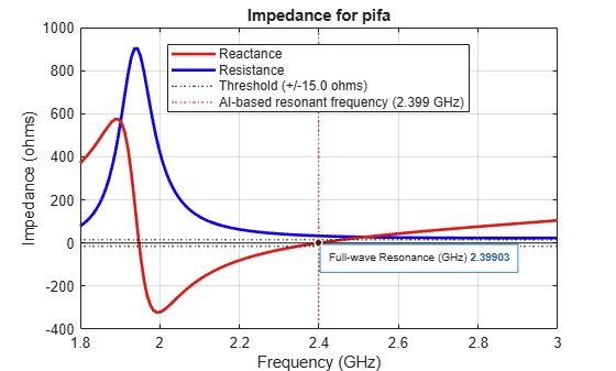
fig = figure;
bandwidth(pifaAnt,fSweep);
compareBandwidth(fig,bandwidthAI,lowerFrequencyAI,upperFrequencyAI)
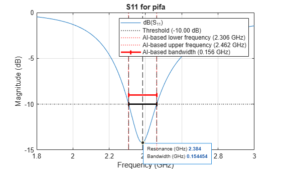
The AI-based analysis is nearly indistinguishable from the full-wave EM solver results, but the AI-based calculations are significantly faster than the full-wave EM solver calculation time.
Now compare the results in a table.
allAIResults = [ ...
    resonantFrequencyAI; ...
    bandwidthAI;
    lowerFrequencyAI;
    upperFrequencyAI;
    ];
allFullResults = [ ...
    resonantFrequencyFull; ...
    bandwidthFull;
    lowerFrequencyFull;
    upperFrequencyFull;
    ];
absErr = abs(allAIResults - allFullResults);
relativeErrorPercent = 100*absErr./allFullResults;
tErr = table(allAIResults,allFullResults,relativeErrorPercent, ...
    RowNames=["resonantFrequency";"bandwidth";"lowerFrequency";"upperFrequency"])
tErr=4×3 table
                         allAIResults    allFullResults    relativeErrorPercent
                         ____________    ______________    ____________________

    resonantFrequency     2.3991e+09        2.399e+09           0.0045166
    bandwidth             1.5564e+08       1.5424e+08             0.90996
    lowerFrequency        2.3063e+09       2.3069e+09            0.029536
    upperFrequency        2.4619e+09       2.4612e+09             0.02934
tTime = table(timeAI,timeFull)
tTime=1×2 table
    timeAI     timeFull
    _______    ________

    0.29349     19.784
Rapidly Explore and Characterize Antenna Across Design Space
Optimize your antenna design by reducing the height by 5%, but maintain the same the resonant frequency, width-to-length and width-to-short pin width ratio, and the existence of the bandwidth. To find the desired length, use AI-based analysis to rapidly explore this design space. [2]
First, define the parameters for tuning the height and length incrementally to characterize the space by using defaultTunableParameters to track the default values. To maintain the resonant frequency, specify the tuning range of the length to be a narrow range, because the length is the resonant dimension [1] and the resonant frequency of your antenna is already relatively close to the desired frequency.
n = 50;
hScaler = linspace(0.86,1.14,n);
lScaler = linspace(0.968,1.032,n);
H0 = pifaAI.defaultTunableParameters.Height;
L0 = pifaAI.defaultTunableParameters.Length;
Keeping the width-to-length ratio locked at 0.7, explore the design space by calculating the resonant frequency with respect to the antenna's height and length. For the sake of maintaining the bandwidth, use the AI-based bandwidth function to verify that the tuned antenna is still matched at 50 ohms.
fResAI = zeros(n);
numNotMatched = 0;
tic
for hIdx = 1:n
    for lIdx = 1:n
        pifaAI.Height = H0*hScaler(hIdx);
        pifaAI.Length = L0*lScaler(lIdx);
        pifaAI.Width = pifaAI.Length*0.7;
        pifaAI.ShortPinWidth = pifaAI.Width;
        [~,~,~,matching] = bandwidth(pifaAI);
        switch string(matching)
            case "Matched"
                fResAI(lIdx,hIdx) = resonantFrequency(pifaAI);
            case {"Almost","Not Matched"}
                fResAI(lIdx,hIdx) = NaN;
                numNotMatched = numNotMatched + 1;
        end
    end
end
timeAI1 = toc;

if numNotMatched >= 1
    disp("Antenna is not matched for " + num2str(numNotMatched) + " geometries. These geometries have been discarded from design space.")
end
Antenna is not matched for 49 geometries. These geometries have been discarded from design space.
Visualize the AI-based calculations of the resonant frequency across the design space.
fig1 = figure;
surf(hScaler*H0*100,lScaler*L0*100,fResAI*1e-9)
view(105,15)
xlabel("Height (cm)")
ylabel("Length (cm)")
zlabel("Resonant Frequency (GHz)")
title(sprintf("Design Space (%1.3f sec)",timeAI1))
Plot where the resonant frequency intersects with the desired value of 2.4 GHz.
hold on
surf(hScaler*H0*100,lScaler*L0*100,ones(n)*fd*1e-9, ...
    FaceAlpha=0)
text(H0*hScaler(end)*100,L0*lScaler(1)*100,fd*1e-9, ...
    strcat("\uparrow",sprintf("\nDesired (%1.1f GHz)\n",fd*1e-9)), ...
    VerticalAlignment="top", ...
    FontWeight="bold")
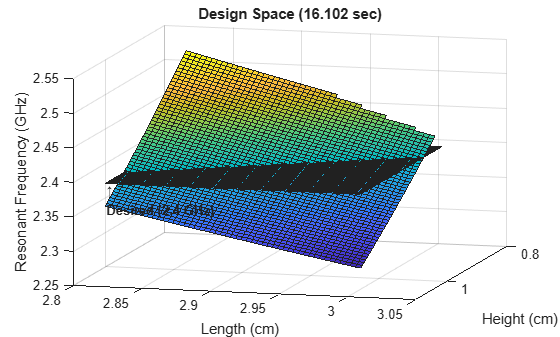
Notice that you were able to calculate 50 * 50 = 2500 points in the design space within a couple of seconds. This would not have been practical using full-wave EM analysis due to the substantially longer computation time.
Examine Response Surface to Identify Desired Design Point
Calculate the desired size-reduced height.
H1 = H0*0.95
H1 =
0.0092
Find the desired length based on this desired height. Inspect the design space to find the point where the resonant frequency is 2.4 GHz and the height is 0.0297978 m.
L1 = 0.0297978;
Calculate the resonant frequency at the desired length and height using AI-based analysis, and visualize the point which the desired length and height was inspected.
pifaAI.Height = H1;
pifaAI.Length = L1;
pifaAI.Width = pifaAI.Length*0.7;
pifaAI.ShortPinWidth = pifaAI.Width;
F1 = resonantFrequency(pifaAI);
s = fig1.CurrentAxes.Children(2);
s.DataTipTemplate.DataTipRows(1).Label = "Height";
s.DataTipTemplate.DataTipRows(2).Label = "Length";
s.DataTipTemplate.DataTipRows(3).Label = "Resonant Frequency";
dt = datatip(s,H1*100,L1*100,F1*1e-9);

Calculate and Analyze Final Design From AI-Based Results
Get your final antenna design along with its analysis results. Throughout this AI-aided optimization process, you have reduced the height of the PIFA while maintaining the existence of the bandwidth and keeping resonant frequency around 2.4 GHz.
lengthFinal = pifaAI.Length;
heightFinal = pifaAI.Height;
widthFinal = pifaAI.Width;

resonantFrequencyFinalAI = F1;
[bandwidthFinalAI,lowerFrequencyFinalAI,upperFrequencyFinalAI] = ...
    bandwidth(pifaAI);

W0 = pifaAI.defaultTunableParameters.Width;

lengthPifa = [lengthFinal;L0];
heightPifa = [heightFinal;H0];
widthPifa = [widthFinal;W0];
resonantFrequencyPifa = [resonantFrequencyFinalAI;resonantFrequencyAI0];
bandwidthPifa = [bandwidthFinalAI;bandwidthAI0];
lowerFrequencyPifa = [lowerFrequencyFinalAI;lowerFrequencyAI0];
upperFrequencyPifa = [upperFrequencyFinalAI;upperFrequencyAI0];
tFinal = table(lengthPifa,heightPifa,widthPifa, ...
    resonantFrequencyPifa,bandwidthPifa,lowerFrequencyPifa,upperFrequencyPifa, ...
    RowNames=["Final Design","Initial Prototype"])
tFinal=2×7 table
                         lengthPifa    heightPifa    widthPifa    resonantFrequencyPifa    bandwidthPifa    lowerFrequencyPifa    upperFrequencyPifa
                         __________    __________    _________    _____________________    _____________    __________________    __________________

    Final Design          0.029798     0.0092324     0.020858          2.3982e+09           1.1813e+08          2.3187e+09            2.4368e+09
    Initial Prototype     0.029167     0.0097183     0.019449          2.4091e+09           1.4809e+08          2.3186e+09            2.4667e+09
Verify AI-Based Results Against Full-Wave EM Simulation
Finally, run the full-wave EM solver on your final antenna.
pifaAntFinal = exportAntenna(pifaAI);

[resonantFrequencyFinalFullAll,~,~,typeAllFull] = resonantFrequency(pifaAntFinal,fSweep);
idxFullFinal = getResonanceCloseToDesign(resonantFrequencyFinalFullAll,typeAllFull,fd,"Series");
resonantFrequencyFinalFull = resonantFrequencyFinalFullAll(idxFullFinal)
resonantFrequencyFinalFull = 2.3990e+09
[bandwidthFinalFull,~,lowerFrequencyFinalFull,upperFrequencyFinalFull] = ...
    bandwidth(pifaAntFinal,fSweep)
bandwidthFinalFull = 1.1840e+08
lowerFrequencyFinalFull =
2.3169e+09
upperFrequencyFinalFull =
2.4353e+09
Verify that the AI-based design of your antenna was accurate by comparing it against the full-wave EM solver results.
allAIResultsFinal = [ ...
    resonantFrequencyFinalAI; ...
    bandwidthFinalAI;
    lowerFrequencyFinalAI;
    upperFrequencyFinalAI;
    ];
allFullResults = [ ...
    resonantFrequencyFinalFull; ...
    bandwidthFinalFull;
    lowerFrequencyFinalFull;
    upperFrequencyFinalFull;
    ];
absErrFinal = abs(allAIResultsFinal - allFullResults);
relativeErrorPercentFinal = 100*absErrFinal./allFullResults;
tErrFinal = table(allAIResultsFinal,allFullResults,relativeErrorPercentFinal, ...
    RowNames=["resonantFrequency";"bandwidth";"lowerFrequency";"upperFrequency"])
tErrFinal=4×3 table
                         allAIResultsFinal    allFullResults    relativeErrorPercentFinal
                         _________________    ______________    _________________________

    resonantFrequency       2.3982e+09           2.399e+09              0.033832
    bandwidth               1.1813e+08           1.184e+08               0.23182
    lowerFrequency          2.3187e+09          2.3169e+09              0.074195
    upperFrequency          2.4368e+09          2.4353e+09              0.059317
Summary of AI-Based Analysis
AI-based analysis allows for the characterization of antennas with:
Faster calculation time
High accuracy
This enables workflows that were not previously practical. As demonstrated in this example, you can explore a design space with high resolution within a couple of seconds.
With AIAntenna, you can take advantage of AI-based analysis without prior machine learning experience.
Reference
[1] Jackson, David. "Chapter 7: Microstrip Antennas," in Antenna Engineering Handbook, edited by John Volakis, 4th ed., New York: McGraw-Hill Co., 2007.
[2] Sivaramakrishnan, Sudarshan, Vishwanath Iyer, Tina Gao, and Giorgia Zucchelli. “A Systematic Application of AI Techniques to Antenna Design, Analysis, and Optimization.” In 2024 54th European Microwave Conference (EuMC), 972–75. Paris, France: IEEE, 2024. https://doi.org/10.23919/EuMC61614.2024.10732562.