Solve Semilinear DAE System

This workflow is an alternative workflow to solving semilinear differential algebraic equations (DAEs), used only if reduceDAEIndex failed in the standard workflow with the warning message: The index of the reduced DAEs is larger than 1. [daetools::reduceDAEIndex]. For the standard workflow, see Solve Differential Algebraic Equations (DAEs).

Complete steps 1 and 2 in Solve Differential Algebraic Equations (DAEs) before beginning other steps. Then, in step 3, if reduceDAEIndex fails, reduce the differential index using reduceDAEToODE. The advantage of reduceDAEToODE is that it reliably reduces semilinear DAEs to ODEs (DAEs of index 0). However, this function is slower and works only on semilinear DAE systems. reduceDAEToODE can fail if the system is not semilinear.

To solve your DAE system, complete these steps.

Step 1. Specify Equations and Variables

The DAE system of equations is:

$$\begin{array}{l}m\frac{d^{2}x}{d{t}^2}=T\left(t\right)\frac{x\left(t\right)}{r}\\ m\frac{d^{2}y}{d{t}^2}=T\left(t\right)\frac{y\left(t\right)}{r}-mg\\ x{\left(t\right)}^2+y{\left(t\right)}^2=r^2\end{array}$$

Specify independent variables and state variables by using syms.

syms x(t) y(t) T(t) m r g

Specify equations by using the == operator.

eqn1 = m*diff(x(t), 2) == T(t)/r*x(t);
eqn2 = m*diff(y(t), 2) == T(t)/r*y(t) - m*g;
eqn3 = x(t)^2 + y(t)^2 == r^2;
eqns = [eqn1 eqn2 eqn3];

Place the state variables in a column vector. Store the number of original variables for reference.

vars = [x(t); y(t); T(t)];
origVars = length(vars);

Step 2. Reduce Differential Order

The differential order of a DAE system is the highest differential order of its equations. To solve DAEs using MATLAB, the differential order must be reduced to 1. Here, the first and second equations have second-order derivatives of x(t) and y(t). Thus, the differential order is 2.

Reduce the system to a first-order system by using reduceDifferentialOrder. The reduceDifferentialOrder function substitutes derivatives with new variables, such as Dxt(t) and Dyt(t). The right side of the expressions in eqns is 0.

[eqns,vars] = reduceDifferentialOrder(eqns,vars)

eqns = 
$$\left(\begin{array}{c}m\hspace{0.17em}\frac{\partial }{\partial t}\mathrm{ }\mathrm{Dxt}\left(t\right)-\frac{T\left(t\right)\hspace{0.17em}x\left(t\right)}{r}\\ g\hspace{0.17em}m+m\hspace{0.17em}\frac{\partial }{\partial t}\mathrm{ }\mathrm{Dyt}\left(t\right)-\frac{T\left(t\right)\hspace{0.17em}y\left(t\right)}{r}\\ -r^2+{x\left(t\right)}^2+{y\left(t\right)}^2\\ \mathrm{Dxt}\left(t\right)-\frac{\partial }{\partial t}\mathrm{ }x\left(t\right)\\ \mathrm{Dyt}\left(t\right)-\frac{\partial }{\partial t}\mathrm{ }y\left(t\right)\end{array}\right)$$

vars = 
$$\left(\begin{array}{c}x\left(t\right)\\ y\left(t\right)\\ T\left(t\right)\\ \mathrm{Dxt}\left(t\right)\\ \mathrm{Dyt}\left(t\right)\end{array}\right)$$

Step 3. Reduce Differential Index with reduceDAEToODE

To reduce the differential index of the DAEs described by eqns and vars, use reduceDAEToODE. To reduce the index, reduceDAEToODE adds new variables and equations to the system. reduceDAEToODE also returns constraints, which are conditions that help find initial values to ensure that the resulting ODEs are equal to the initial DAEs.

[ODEs,constraints] = reduceDAEToODE(eqns,vars)

ODEs = 
$$\left(\begin{array}{c}\mathrm{Dxt}\left(t\right)-\frac{\partial }{\partial t}\mathrm{ }x\left(t\right)\\ \mathrm{Dyt}\left(t\right)-\frac{\partial }{\partial t}\mathrm{ }y\left(t\right)\\ m\hspace{0.17em}\frac{\partial }{\partial t}\mathrm{ }\mathrm{Dxt}\left(t\right)-\frac{T\left(t\right)\hspace{0.17em}x\left(t\right)}{r}\\ m\hspace{0.17em}\frac{\partial }{\partial t}\mathrm{ }\mathrm{Dyt}\left(t\right)-\frac{T\left(t\right)\hspace{0.17em}y\left(t\right)-g\hspace{0.17em}m\hspace{0.17em}r}{r}\\ -\left(4\hspace{0.17em}T\left(t\right)\hspace{0.17em}y\left(t\right)-2\hspace{0.17em}g\hspace{0.17em}m\hspace{0.17em}r\right)\hspace{0.17em}\frac{\partial }{\partial t}\mathrm{ }y\left(t\right)-\left(2\hspace{0.17em}{x\left(t\right)}^2+2\hspace{0.17em}{y\left(t\right)}^2\right)\hspace{0.17em}\frac{\partial }{\partial t}\mathrm{ }T\left(t\right)-4\hspace{0.17em}T\left(t\right)\hspace{0.17em}x\left(t\right)\hspace{0.17em}\frac{\partial }{\partial t}\mathrm{ }x\left(t\right)-4\hspace{0.17em}m\hspace{0.17em}r\hspace{0.17em}\mathrm{Dxt}\left(t\right)\hspace{0.17em}\frac{\partial }{\partial t}\mathrm{ }\mathrm{Dxt}\left(t\right)-4\hspace{0.17em}m\hspace{0.17em}r\hspace{0.17em}\mathrm{Dyt}\left(t\right)\hspace{0.17em}\frac{\partial }{\partial t}\mathrm{ }\mathrm{Dyt}\left(t\right)\end{array}\right)$$

constraints = 
$$\left(\begin{array}{c}-2\hspace{0.17em}m\hspace{0.17em}r\hspace{0.17em}{\mathrm{Dxt}\left(t\right)}^2-2\hspace{0.17em}m\hspace{0.17em}r\hspace{0.17em}{\mathrm{Dyt}\left(t\right)}^2-2\hspace{0.17em}T\left(t\right)\hspace{0.17em}{x\left(t\right)}^2-2\hspace{0.17em}T\left(t\right)\hspace{0.17em}{y\left(t\right)}^2+2\hspace{0.17em}g\hspace{0.17em}m\hspace{0.17em}r\hspace{0.17em}y\left(t\right)\\ r^2-{x\left(t\right)}^2-{y\left(t\right)}^2\\ 2\hspace{0.17em}\mathrm{Dxt}\left(t\right)\hspace{0.17em}x\left(t\right)+2\hspace{0.17em}\mathrm{Dyt}\left(t\right)\hspace{0.17em}y\left(t\right)\end{array}\right)$$

Step 4. ODEs to Function Handles for ode15s and ode23t

From the output of reduceDAEToODE, you have a vector of equations in ODEs and a vector of variables in vars. To use ode15s or ode23t, you need two function handles: one representing the mass matrix of the ODE system, and the other representing the vector containing the right sides of the mass matrix equations. These function handles are the equivalent mass matrix representation of the ODE system where M(t,y(t))y’(t) = f(t,y(t)).

Find these function handles by using massMatrixForm to get the mass matrix massM (M in the equation) and right sides f.

[massM,f] = massMatrixForm(ODEs,vars)

massM = 
$$\left(\begin{array}{ccccc}-1& 0& 0& 0& 0\\ 0& -1& 0& 0& 0\\ 0& 0& 0& m& 0\\ 0& 0& 0& 0& m\\ -4\hspace{0.17em}T\left(t\right)\hspace{0.17em}x\left(t\right)& 2\hspace{0.17em}g\hspace{0.17em}m\hspace{0.17em}r-4\hspace{0.17em}T\left(t\right)\hspace{0.17em}y\left(t\right)& -2\hspace{0.17em}{x\left(t\right)}^2-2\hspace{0.17em}{y\left(t\right)}^2& -4\hspace{0.17em}m\hspace{0.17em}r\hspace{0.17em}\mathrm{Dxt}\left(t\right)& -4\hspace{0.17em}m\hspace{0.17em}r\hspace{0.17em}\mathrm{Dyt}\left(t\right)\end{array}\right)$$

f = 
$$\left(\begin{array}{c}-\mathrm{Dxt}\left(t\right)\\ -\mathrm{Dyt}\left(t\right)\\ \frac{T\left(t\right)\hspace{0.17em}x\left(t\right)}{r}\\ \frac{T\left(t\right)\hspace{0.17em}y\left(t\right)-g\hspace{0.17em}m\hspace{0.17em}r}{r}\\ 0\end{array}\right)$$

The equations in ODEs can contain symbolic parameters that are not specified in the vector of variables vars. Find these parameters by using setdiff on the output of symvar from ODEs and vars.

pODEs = symvar(ODEs);
pvars = symvar(vars);
extraParams = setdiff(pODEs, pvars)

extraParams = $$\left(\begin{array}{ccc}g& m& r\end{array}\right)$$

The extra parameters that you need to specify are the mass m, radius r, and gravitational constant g.

Convert massM and f to function handles using odeFunction. Specify the extra symbolic parameters as additional inputs to odeFunction.

massM = odeFunction(massM, vars, m, r, g);
f = odeFunction(f, vars, m, r, g);

The rest of the workflow is purely numerical. Set the parameter values and substitute the parameter values in DAEs and constraints.

m = 1;
r = 1;
g = 9.81;
ODEsNumeric = subs(ODEs);
constraintsNumeric = subs(constraints);

Create the function handle suitable for input to ode15s or ode23s.

M = @(t,Y) massM(t,Y,m,r,g);
F = @(t,Y) f(t,Y,m,r,g);

Step 5. Initial Conditions for ode15s and ode23t

The solvers require initial values for all variables in the function handle. Find initial values that satisfy the equations by using the MATLAB® decic function. The decic accepts guesses (which might not satisfy the equations) for the initial conditions and tries to find satisfactory initial conditions using those guesses. decic can fail, in which case you must manually supply consistent initial values for your problem.

First, check the variables in vars.

vars

vars = 
$$\left(\begin{array}{c}x\left(t\right)\\ y\left(t\right)\\ T\left(t\right)\\ \mathrm{Dxt}\left(t\right)\\ \mathrm{Dyt}\left(t\right)\end{array}\right)$$

Here, Dxt(t) is the first derivative of x(t), and so on. There are 5 variables in a 5-by-1 vector. Therefore, guesses for initial values of variables and their derivatives must also be 5-by-1 vectors.

Assume the initial angular displacement of the pendulum is 30° or pi/6, and the origin of the coordinates is at the suspension point of the pendulum. Given that we used a radius r of 1, the initial horizontal position x(t) is r*sin(pi/6). The initial vertical position y(t) is -r*cos(pi/6). Specify these initial values of the variables in the vector y0est.

Arbitrarily set the initial values of the remaining variables and their derivatives to 0. These are not good guesses. However, they suffice for this problem. In your problem, if decic errors, then provide better guesses and refer to the decic page.

y0est = [r*sin(pi/6); -r*cos(pi/6); 0; 0; 0];
yp0est = zeros(5,1);

Create an option set that contains the mass matrix M of the system and specifies numerical tolerances for the numerical search.

opt = odeset('Mass', M, 'RelTol', 10.0^(-7), 'AbsTol' , 10.0^(-7));

Find initial values consistent with the system of ODEs and with the algebraic constraints by using decic. The parameter [1,0,0,0,1] in this function call fixes the first and the last element in y0est, so that decic does not change them during the numerical search. Here, this fixing is necessary to ensure decic finds satisfactory initial conditions.

[y0, yp0] = decic(ODEsNumeric, vars, constraintsNumeric, 0,...
                y0est, [1,0,0,0,1], yp0est, opt)

y0 = 5×1

    0.5000
   -0.8660
   -8.4957
         0
         0

yp0 = 5×1

         0
         0
         0
   -4.2479
   -2.4525

Now create an option set that contains the mass matrix M of the system and the vector yp0 of consistent initial values for the derivatives. You will use this option set when solving the system.

opt = odeset(opt, 'InitialSlope', yp0);

Step 6. Solve an ODE System with ode15s or ode23t

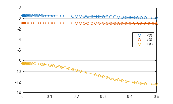
Solve the system integrating over the time span 0 ≤ t ≤ 0.5. Add the grid lines and the legend to the plot. Use ode23s by replacing ode15s with ode23s.

[tSol,ySol] = ode15s(F, [0, 0.5], y0, opt);
plot(tSol,ySol(:,1:origVars),'-o')

for k = 1:origVars
  S{k} = char(vars(k));
end

legend(S, 'Location', 'Best')
grid on

Solve the system for different parameter values by setting the new value and regenerating the function handle and initial conditions.

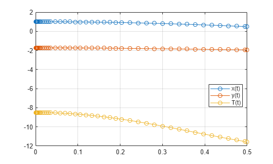
Set r to 2 and repeat the steps.

r = 2;

ODEsNumeric = subs(ODEs);
constraintsNumeric = subs(constraints);
M = @(t,Y) massM(t,Y,m,r,g);
F = @(t,Y) f(t,Y,m,r,g);

y0est = [r*sin(pi/6); -r*cos(pi/6); 0; 0; 0];
opt = odeset('Mass', M, 'RelTol', 10.0^(-7), 'AbsTol' , 10.0^(-7));
[y0, yp0] = decic(ODEsNumeric, vars, constraintsNumeric, 0,...
		 y0est, [1,0,0,0,1], yp0est, opt);

opt = odeset(opt, 'InitialSlope', yp0);

Solve the system for the new parameter value.

[tSol,ySol] = ode15s(F, [0, 0.5], y0, opt);
plot(tSol,ySol(:,1:origVars),'-o')

for k = 1:origVars
  S{k} = char(vars(k));
end

legend(S, 'Location', 'Best')
grid on