주요 콘텐츠

smoteTabularSynthesizer

SMOTE-based synthesizer for tabular data synthesis

Since R2026a

    Description

    To generate synthetic data, you can first create a smoteTabularSynthesizer object using an existing multivariate data set. Then, use the synthesizeTabularData object function to synthesize data using SMOTE (synthetic minority oversampling technique). After you synthesize data, you can test whether the new data set comes from the same distribution as the original data set. Use the mmdtest or knntest function to determine how close the data distributions are to each other. For more information about SMOTE, see Generate Synthetic Data Using SMOTE.

    Creation

    Description

    synthesizer = smoteTabularSynthesizer(X) creates a SMOTE-based synthesizer object (synthesizer) using the existing data X.

    synthesizer = smoteTabularSynthesizer(X,Yname) creates a synthesizer object using the existing data in the table X and the class labels variable Yname in X.

    example

    synthesizer = smoteTabularSynthesizer(X,Y) creates a synthesizer object using the existing data X and the class labels Y.

    synthesizer = smoteTabularSynthesizer(___,Name=Value) specifies options using one or more name-value arguments in addition to any of the input argument combinations in the previous syntaxes. For example, you can specify the number of nearest neighbors and the variables to use to generate synthetic data.

    Input Arguments

    expand all

    Existing data set, specified as a numeric matrix or a table. Rows of X correspond to observations, and columns of X correspond to variables. Multicolumn variables and cell arrays other than cell arrays of character vectors are not supported.

    Data Types: single | double | table

    Name of the class labels variable in X, specified as a character vector or string scalar. X must be a table, and Yname must specify a column in X that is a numeric, categorical, or logical vector; a character or string array; or a cell array of character vectors. The Yname variable must contain class labels for one or two classes only.

    Data Types: char | string

    Class labels for one or two classes, specified as a numeric, categorical, or logical vector; a character or string array; or a cell array of character vectors. Rows of Y correspond to observations.

    Data Types: single | double | logical | char | string | cell | categorical

    Name-Value Arguments

    expand all

    Specify optional pairs of arguments as Name1=Value1,...,NameN=ValueN, where Name is the argument name and Value is the corresponding value. Name-value arguments must appear after other arguments, but the order of the pairs does not matter.

    Example: smoteTabularSynthesizer(X,Y,NumNeighbors=3,Distance="fastseuclidean") specifies to use 3 nearest neighbors and the fast standardized Euclidean distance.

    Number of nearest neighbors to use when generating synthetic data, specified as a positive integer scalar.

    • If you do not specify Yname or Y, the default value for NumNeighbors is min(5,size(X,1)).

    • If you specify Yname or Y, the default value for NumNeighbors is a scalar or two-element vector. Each entry is min(5,n), where n is the number of observations in the corresponding class.

    Example: NumNeighbors=10

    Data Types: single | double

    Distance metric for finding nearest neighbors, specified as a character vector or string scalar.

    • If all the variables are continuous (numeric), then you can specify one of the following distance metrics.

      ValueDescription
      "euclidean"

      Euclidean distance

      "fasteuclidean"Euclidean distance computed by using an alternative algorithm that saves time when the number of variables is at least 10. In some cases, this faster algorithm can reduce accuracy.
      "seuclidean"

      Standardized Euclidean distance. Each coordinate difference between observations is scaled by dividing by the corresponding variable standard deviation.

      "fastseuclidean"Standardized Euclidean distance computed by using an alternative algorithm that saves time when the number of variables is at least 10. In some cases, this faster algorithm can reduce accuracy.

      Note

      If you specify one of these distance metrics and the data includes categorical variables, then the software treats each categorical variable as a numeric variable for the distance computation, with each category represented by a positive integer.

    • If all the variables are categorical, then you can specify the following distance metric.

      ValueDescription
      "hamming"

      Hamming distance, which is the percentage of coordinates that differ

      Note

      If you specify this distance metric and the data includes continuous (numeric) variables, then the software treats each continuous variable as a categorical variable for the distance computation.

    • If the variables are a mix of continuous (numeric) and categorical variables, then you can specify the following distance metric.

      ValueDescription
      "goodall3"

      Modified Goodall distance

    The default value is "seuclidean" if all the variables are continuous, "hamming" if all the variables are categorical, and "goodall3" if the variables are a mix of continuous and categorical variables.

    Example: Distance="euclidean"

    Data Types: char | string

    Size in megabytes of the cache allocated for the distance computation, specified as "maximal" or a positive scalar. If the cache size is "maximal", the software tries to allocate enough memory for an intermediate matrix.

    The CacheSize name-value argument is valid only when the Distance value is "fasteuclidean", "fastseuclidean", or "goodall3".

    • For the fast distance metrics, the intermediate matrix corresponds to the Gram matrix.

    • For the modified Goodall distance metric, the intermediate matrix corresponds to the distance matrix.

    Example: CacheSize="maximal"

    Data Types: single | double | char | string

    Variable names, specified as a string array or a cell array of character vectors.

    • If X is a numeric matrix, then you can use VariableNames to assign names to the variables in X.

      • The order of the names in VariableNames must correspond to the order of the variables in X. That is, VariableNames{1} is the name of X(:,1), VariableNames{2} is the name of X(:,2), and so on. size(X,2) and numel(VariableNames) must be equal.

      • By default, VariableNames is {'x1','x2',...}.

    • If X is a table, then you can use VariableNames to specify which variables to use. That is, smoteTabularSynthesizer uses only the variables in VariableNames to generate synthetic data.

      • VariableNames must be a subset of X.Properties.VariableNames.

      • By default, VariableNames contains the names of all variables, excluding the class labels variable Yname.

    Example: VariableNames=["SepalLength","SepalWidth","PetalLength","PetalWidth"]

    Data Types: string | cell

    List of the categorical variables, excluding the class labels variable Yname, specified as one of the values in this table.

    ValueDescription
    Positive integer vector

    Each entry in the vector is an index value indicating that the corresponding variable is categorical. The index values are between 1 and v, where v is the number of variables listed in VariableNames.

    Logical vector

    A true entry means that the corresponding variable is categorical. The length of the vector is v.

    String array or cell array of character vectorsEach element in the array is the name of a categorical variable. The names must match the entries in VariableNames.
    "all"All variables are categorical.

    By default, if the variables are in a numeric matrix, the software assumes all the variables are continuous. If the variables are in a table, the software assumes they are categorical if they are logical vectors, categorical vectors, character arrays, string arrays, or cell arrays of character vectors. To identify any other variables as categorical, specify them by using the CategoricalVariables name-value argument.

    Do not specify discrete numeric variables as categorical variables. Use the DiscreteNumericVariables name-value argument instead.

    Example: CategoricalVariables="all"

    Data Types: single | double | logical | string | cell

    List of the discrete numeric variables, specified as one of the values in this table.

    ValueDescription
    Positive integer vector

    Each entry in the vector is an index value indicating that the corresponding variable is a discrete numeric variable. The index values are between 1 and v, where v is the number of variables listed in VariableNames.

    Logical vector

    A true entry means that the corresponding variable is a discrete numeric variable. The length of the vector is v.

    String array or cell array of character vectorsEach element in the array is the name of a discrete numeric variable. The names must match the entries in VariableNames.
    "all"All variables are discrete numeric variables.

    You cannot specify categorical variables as discrete numeric variables.

    Example: DiscreteNumericVariables=[2 5]

    Data Types: single | double | logical | string | cell

    Properties

    expand all

    This property is read-only.

    Variable names, returned as a string array. The order of the elements of VariableNames corresponds to the order in which the variable names appear in the existing data set X.

    Data Types: string

    This property is read-only.

    Indices of the categorical variables, returned as a positive integer vector. Each index value in CategoricalVariables indicates that the corresponding variable listed in VariableNames is categorical. If none of the variables are categorical, then this property is empty ([]).

    Data Types: double

    This property is read-only.

    Indices of the discrete numeric variables, returned as a positive integer vector. Each index value in DiscreteNumericVariables indicates that the corresponding variable listed in VariableNames is a discrete numeric variable. If none of the variables are discrete numeric variables, then this property is empty ([]).

    Data Types: double

    This property is read-only.

    Number of nearest neighbors to use when generating synthetic data, returned as a positive integer scalar or a two-element positive integer vector. If you specify class labels when you create the synthesizer object, then NumNeighbors(i) corresponds to the number of nearest neighbors to use for class ClassNames(i,:).

    Data Types: single | double

    This property is read-only.

    Distance metric used for finding nearest neighbors, returned as "euclidean", "fasteuclidean", "fastseuclidean", "goodall3", "hamming", or "seuclidean". For more information on these distance metrics, see the Distance name-value argument.

    Data Types: string

    This property is read-only.

    Names of the classes in Yname or Y for which to generate synthetic data, returned as a numeric, categorical, or logical vector; a character or string array; or a cell array of character vectors. If you do not specify class labels when you create the synthesizer object, then this property is empty ([]).

    Data Types: single | double | logical | char | string | cell | categorical

    This property is read-only.

    Number of observations in the existing data set X, returned as a positive integer scalar or a two-element positive integer vector. If you specify class labels when you create the synthesizer object, then NumObservations(i) corresponds to the number of observations in the existing data set that belong to class ClassNames(i,:).

    Data Types: double

    Object Functions

    synthesizeTabularDataSynthesize tabular data using binning-based or SMOTE-based synthesizer

    Examples

    collapse all

    Use existing training data to create a smoteTabularSynthesizer object. Then, synthesize data using the synthesizeTabularData object function. Train a model using the existing training data, and then train the same type of model using both the existing training data and the synthetic data. Compare the performance of the two models using test data.

    Load the carbig data set, which contains measurements of cars made in the 1970s and early 1980s. Categorize the cars based on whether they were made in Europe.

    load carbig
    Origin = categorical(cellstr(Origin));
    Origin = mergecats(Origin,["France","Germany", ...
        "Sweden","Italy","England"],"Europe");
    Origin = mergecats(Origin,["USA","Japan"],"NotEurope");
    tabulate(Origin)
          Value    Count   Percent
         Europe       73     17.98%
      NotEurope      333     82.02%
    

    The data is imbalanced, with only about 18% of cars originating in Europe.

    Create a table containing the variables Acceleration, Displacement, and so on, as well as the response variable Origin. Remove rows of cars where the table has missing values.

    cars = table(Acceleration,Displacement,Horsepower, ...
        MPG,Weight,Origin);
    cars = rmmissing(cars);

    Partition the data into training and test sets. Use approximately 50% of the observations for model training and synthesizing new data, and 50% of the observations for model testing. Use stratified partitioning so that approximately the same ratio of European to non-European cars exists in both the training and test sets.

    rng("default")
    cv = cvpartition(cars.Origin,Holdout=0.5);
    trainCars = cars(training(cv),:);
    testCars = cars(test(cv),:);

    Create a smoteTabularSynthesizer object using the trainCars data set. Specify Origin as the class labels variable.

    synthesizer = smoteTabularSynthesizer(trainCars,"Origin")
    synthesizer = 
      smoteTabularSynthesizer
    
          VariableNames: ["Acceleration"    "Displacement"    "Horsepower"    "MPG"    "Weight"]
             ClassNames: [Europe    NotEurope]
           NumNeighbors: [5 5]
               Distance: "seuclidean"
        NumObservations: [34 162]
    
    
      Properties, Methods


    synthesizer is a smoteTabularSynthesizer object with two classes (Europe and NotEurope).

    Synthesize new data by using synthesizer. Specify to generate 40 observations belonging to the class of European cars only.

    syntheticCars = synthesizeTabularData(synthesizer,40,ClassNames="Europe");

    The synthesizeTabularData object function uses the information stored in synthesizer to generate syntheticCars.

    To visualize the difference between the existing European car data and the synthetic European car data, you can use the detectdrift function. Filter the trainCars data to include European car data only. The detectdrift function uses permutation testing to detect drift between europeanCars and syntheticCars.

    europeanCars = trainCars(trainCars.Origin=="Europe",:);
    
    dd = detectdrift(europeanCars,syntheticCars);

    dd is a DriftDiagnostics object with a plotEmpiricalCDF object function for visualization.

    For the continuous variables, use the plotEmpiricalCDF function to see the difference between the empirical cumulative distribution function (ecdf) of the values in europeanCars and the ecdf of the values in syntheticCars.

    continuousVariable = "Acceleration";
    plotEmpiricalCDF(dd,Variable=continuousVariable)
    legend(["Real data","Synthetic data"])

    Figure contains an axes object. The axes object with title ECDF for Acceleration, xlabel Acceleration, ylabel Cumulative Probability contains 2 objects of type stair. These objects represent Real data, Synthetic data.

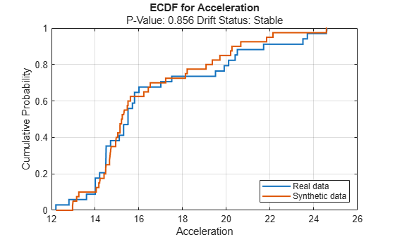
    For the Acceleration predictor, the ecdf plot for the existing values (in blue) matches the ecdf plot for the synthetic values (in red) fairly well.

    Train an SVM classifier using the original training data trainCars. Specify Origin as the response variable, and standardize the predictors before training. Then, train the same kind of classifier using both the original data and the synthetic data (syntheticCars).

    originalMdl = fitcsvm(trainCars,"Origin",Standardize=true);
    newMdl = fitcsvm([trainCars;syntheticCars],"Origin",Standardize=true);

    Evaluate the performance of the two models on the test set using confusion matrices.

    originalPredictions = predict(originalMdl,testCars);
    newPredictions = predict(newMdl,testCars);
    
    tiledlayout(1,2)
    nexttile
    confusionchart(testCars.Origin,originalPredictions)
    title("Original Model")
    nexttile
    confusionchart(testCars.Origin,newPredictions)
    title("New Model")

    Figure contains objects of type ConfusionMatrixChart. The chart of type ConfusionMatrixChart has title Original Model. The chart of type ConfusionMatrixChart has title New Model.

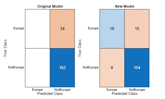
    The model trained on the original data classifies all test observations as non-European cars. The model trained on the original and synthetic data has greater accuracy than the other model and correctly classifies the majority of European cars in the test set.

    Evaluate data synthesized from an existing data set. Compare the existing and synthetic data sets for each class to determine the similarity between the two multivariate data distributions.

    Load the sample file fisheriris.csv, which contains iris data including sepal length, sepal width, petal width, and species type. Read the file into a table, and then display the first eight observations in the table.

    fisheriris = readtable("fisheriris.csv");
    head(fisheriris)
        SepalLength    SepalWidth    PetalLength    PetalWidth     Species  
        ___________    __________    ___________    __________    __________
    
            5.1           3.5            1.4           0.2        {'setosa'}
            4.9             3            1.4           0.2        {'setosa'}
            4.7           3.2            1.3           0.2        {'setosa'}
            4.6           3.1            1.5           0.2        {'setosa'}
              5           3.6            1.4           0.2        {'setosa'}
            5.4           3.9            1.7           0.4        {'setosa'}
            4.6           3.4            1.4           0.3        {'setosa'}
              5           3.4            1.5           0.2        {'setosa'}
    

    Display the types of irises in the table and their proportion in the data set.

    tabulate(fisheriris.Species)
           Value    Count   Percent
          setosa       50     33.33%
      versicolor       50     33.33%
       virginica       50     33.33%
    

    The data set contains three types of irises (setosa, versicolor, and virginica) with 50 observations each.

    Create separate tables for the versicolor data and the virginica data. Combine the two tables into one.

    versicolorData = fisheriris(fisheriris.Species=="versicolor",:);
    virginicaData = fisheriris(fisheriris.Species=="virginica",:);
    irisData = [versicolorData;virginicaData]
    irisData=100×5 table
        SepalLength    SepalWidth    PetalLength    PetalWidth       Species    
        ___________    __________    ___________    __________    ______________
    
              7           3.2            4.7           1.4        {'versicolor'}
            6.4           3.2            4.5           1.5        {'versicolor'}
            6.9           3.1            4.9           1.5        {'versicolor'}
            5.5           2.3              4           1.3        {'versicolor'}
            6.5           2.8            4.6           1.5        {'versicolor'}
            5.7           2.8            4.5           1.3        {'versicolor'}
            6.3           3.3            4.7           1.6        {'versicolor'}
            4.9           2.4            3.3             1        {'versicolor'}
            6.6           2.9            4.6           1.3        {'versicolor'}
            5.2           2.7            3.9           1.4        {'versicolor'}
              5             2            3.5             1        {'versicolor'}
            5.9             3            4.2           1.5        {'versicolor'}
              6           2.2              4             1        {'versicolor'}
            6.1           2.9            4.7           1.4        {'versicolor'}
            5.6           2.9            3.6           1.3        {'versicolor'}
            6.7           3.1            4.4           1.4        {'versicolor'}
          ⋮


    Create 200 new observations from the data in irisData: 100 for the versicolor class and 100 for the virginica class. First, create an object by using the smoteTabularSynthesizer function. Then, synthesize the data by using the synthesizeTabularData object function.

    To better compare class-specific data later on, call the synthesizeTabularData function twice and return versicolor and virginica synthetic data separately.

    synthesizer = smoteTabularSynthesizer(irisData,"Species");
    syntheticVersicolorData = synthesizeTabularData(synthesizer,100, ...
        ClassNames="versicolor");
    syntheticVirginicaData = synthesizeTabularData(synthesizer,100, ...
        ClassNames="virginica");

    For each type of iris, visually compare the observations in the existing data set and the synthetic data set by using scatter plots. Each point corresponds to an observation. The point color indicates the species of the corresponding iris (blue for versicolor and red for virginica).

    tiledlayout(2,2)
    
    nexttile
    scatter(versicolorData,"SepalLength","PetalLength")
    title("Existing Versicolor Data")
    nexttile
    scatter(syntheticVersicolorData,"SepalLength","PetalLength")
    title("Synthetic Versicolor Data")
    
    nexttile
    scatter(virginicaData,"SepalLength","PetalLength", ...
        MarkerEdgeColor="red")
    title("Existing Virginica Data")
    nexttile
    scatter(syntheticVirginicaData,"SepalLength","PetalLength", ...
        MarkerEdgeColor="red")
    title("Synthetic Virginica Data")

    Figure contains 4 axes objects. Axes object 1 with title Existing Versicolor Data, xlabel SepalLength, ylabel PetalLength contains an object of type scatter. Axes object 2 with title Synthetic Versicolor Data, xlabel SepalLength, ylabel PetalLength contains an object of type scatter. Axes object 3 with title Existing Virginica Data, xlabel SepalLength, ylabel PetalLength contains an object of type scatter. Axes object 4 with title Synthetic Virginica Data, xlabel SepalLength, ylabel PetalLength contains an object of type scatter.

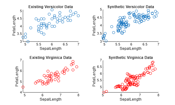
    For each iris type, the scatter plots indicate that the existing data set and the synthetic data set have similar characteristics.

    For each iris type, compare the existing and synthetic data sets by using the knntest function. The function performs a two-sample hypothesis test for the null hypothesis that the data sets come from the same distribution.

    [knnstat1,p1,h1] = knntest(versicolorData,syntheticVersicolorData)
    knnstat1 = 
    0.5327
    
    p1 = 
    0.8830
    
    h1 = 
    0
    
    [knnstat2,p2,h2] = knntest(virginicaData,syntheticVirginicaData)
    knnstat2 = 
    0.5400
    
    p2 = 
    0.7738
    
    h2 = 
    0
    

    For each iris type, the returned value of h = 0 indicates that knntest fails to reject the null hypothesis that the existing data set and the synthetic data set come from different distributions at the 5% significance level. As with other hypothesis tests, this result does not guarantee that the null hypothesis is true. That is, the data sets do not necessarily come from the same distribution, but the high p-value indicates that the distributions of the existing and synthetic data sets are similar.

    Algorithms

    expand all

    References

    [1] Chawla, Nitesh V., Kevin W. Bowyer, Lawrence O. Hall, and W. Philip Kegelmeyer. "SMOTE: Synthetic Minority Over-sampling Technique." Journal of Artificial Intelligence Research 16 (2002): 321-357.

    Version History

    Introduced in R2026a