plotResiduals

Plot residuals of linear mixed-effects model

Syntax

plotResiduals(lme,plottype)

plotResiduals(lme,plottype,Name,Value)

h = plotResiduals(___)

Description

plotResiduals(lme,plottype) plots the raw conditional residuals of the linear mixed-effects model lme in a plot of the type specified by plottype.

example

plotResiduals(lme,plottype,Name,Value) also plots the residuals of the linear mixed-effects model lme with additional options specified by one or more name-value pair arguments. For example, you can specify the residual type to plot.

plotResiduals also accepts some other name-value pair arguments that specify the properties of the primary line in the plot. For those name-value pairs, see plot.

h = plotResiduals(___) returns a handle, h, to the lines or patches in the plot of residuals.

Input Arguments

expand all

`lme` — Linear mixed-effects model
`LinearMixedModel` object

Linear mixed-effects model, specified as a LinearMixedModel object constructed using fitlme or fitlmematrix.

`plottype` — Type of residual plot
`'histogram'` (default) | `'caseorder'` | `'fitted'` | `'lagged'` | `'probability'` | `'symmetry'`

Type of residual plot, specified as one of the following.

`'histogram'`	Default. Histogram of residuals
`'caseorder'`	Residuals versus case (row) order
`'fitted'`	Residuals versus fitted values
`'lagged'`	Residuals versus lagged residual (r(t) versus r(t – 1))
`'probability'`	Normal probability plot
`'symmetry'`	Symmetry plot

Example: plotResiduals(lme,'lagged')

Name-Value Arguments

Specify optional pairs of arguments as Name1=Value1,...,NameN=ValueN, where Name is the argument name and Value is the corresponding value. Name-value arguments must appear after other arguments, but the order of the pairs does not matter.

Before R2021a, use commas to separate each name and value, and enclose Name in quotes.

`ResidualType` — Residual type
`'Raw'` (default) | `'Pearson'` | `'Standardized'`

Residual type, specified by the comma-separated pair consisting of ResidualType and one of the following.

Residual Type Conditional Marginal

Residual Type	Conditional	Marginal
`'Raw'`	$r_{i}^{C} = {[y - X \hat{β} - Z \hat{b}]}_{i}$	$r_{i}^{M} = {[y - X \hat{β}]}_{i}$
`'Pearson'`	$p r_{i}^{C} = \frac{r_{i}^{C}}{{\sqrt{[{\hat{V a r}}_{y, b} (y - X β - Z b)]}}_{i i}}$	$p r_{i}^{M} = \frac{r_{i}^{M}}{\sqrt{{[{\hat{V a r}}_{y} (y - X β)]}_{i i}}}$
`'Standardized'`	$s t_{i}^{C} = \frac{r_{i}^{C}}{\sqrt{{[{\hat{V a r}}_{y} (r^{C})]}_{i i}}}$	$s t_{i}^{M} = \frac{r_{i}^{M}}{\sqrt{{[{\hat{V a r}}_{y} (r^{M})]}_{i i}}}$

'Raw'

$r_{i}^{C} = {[y - X \hat{β} - Z \hat{b}]}_{i}$

$r_{i}^{M} = {[y - X \hat{β}]}_{i}$

'Pearson'

$p r_{i}^{C} = \frac{r_{i}^{C}}{{\sqrt{[{\hat{V a r}}_{y, b} (y - X β - Z b)]}}_{i i}}$

$p r_{i}^{M} = \frac{r_{i}^{M}}{\sqrt{{[{\hat{V a r}}_{y} (y - X β)]}_{i i}}}$

'Standardized'

$s t_{i}^{C} = \frac{r_{i}^{C}}{\sqrt{{[{\hat{V a r}}_{y} (r^{C})]}_{i i}}}$

$s t_{i}^{M} = \frac{r_{i}^{M}}{\sqrt{{[{\hat{V a r}}_{y} (r^{M})]}_{i i}}}$

For more information on the conditional and marginal residuals and residual variances, see Definitions at the end of this page.

Example: 'ResidualType','Standardized'

Output Arguments

expand all

`h` — Handle to residual plot
handle

Handle to the residual plot, returned as a handle.

Examples

expand all

Examine Residuals

Open Live Script

Load the sample data.

load('weight.mat')

weight contains data from a longitudinal study, where 20 subjects are randomly assigned to 4 exercise programs, and their weight loss is recorded over six 2-week time periods. This is simulated data.

Store the data in a table. Define Subject and Program as categorical variables.

tbl = table(InitialWeight,Program,Subject,Week,y);
tbl.Subject = categorical(tbl.Subject);
tbl.Program = categorical(tbl.Program);

Fit a linear mixed-effects model where the initial weight, type of program, week, and the interaction between the week and type of program are the fixed effects. The intercept and week vary by subject.

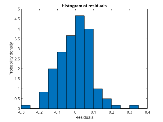
lme = fitlme(tbl,'y ~ InitialWeight + Program*Week + (Week|Subject)');

Plot the histogram of the raw residuals.

plotResiduals(lme)

Figure contains an axes object. The axes object with title Histogram of residuals, xlabel Residuals, ylabel Probability density contains an object of type patch.

Plot the residuals versus the fitted values.

plotResiduals(lme,'fitted')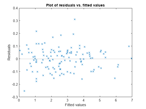

Figure contains an axes object. The axes object with title Plot of residuals vs. fitted values, xlabel Fitted values, ylabel Residuals contains 2 objects of type line. One or more of the lines displays its values using only markers

There is no obvious pattern, so there are no immediate signs of heteroscedasticity.

Create the normal probability plot of residuals.

plotResiduals(lme,'probability')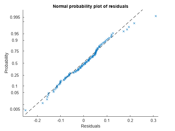

Figure contains an axes object. The axes object with title Normal probability plot of residuals, xlabel Residuals, ylabel Probability contains 2 objects of type line. One or more of the lines displays its values using only markers

Data appears to be normal.

Find the observation number for the data that appears to be an outlier to the right of the plot.

find(residuals(lme)>0.25)

ans = 101

Create a box plot of the raw, Pearson, and standardized residuals.

r = residuals(lme);
pr = residuals(lme,'ResidualType','Pearson');
st = residuals(lme,'ResidualType','Standardized');
X = [r pr st];
boxplot(X,'labels',{'Raw','Pearson','Standardized'})

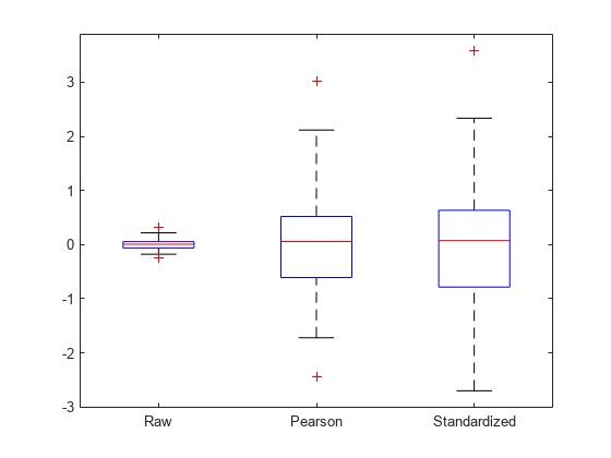
Figure contains an axes object. The axes object contains 21 objects of type line. One or more of the lines displays its values using only markers

All three box plots point out the outlier on the right tail of the distribution. The box plots of raw and Pearson residuals also point out a second possible outlier on the left tail. Find the corresponding observation number.

find(pr<-2)

ans = 10

Plot the raw residuals versus lagged residuals.

plotResiduals(lme,'lagged')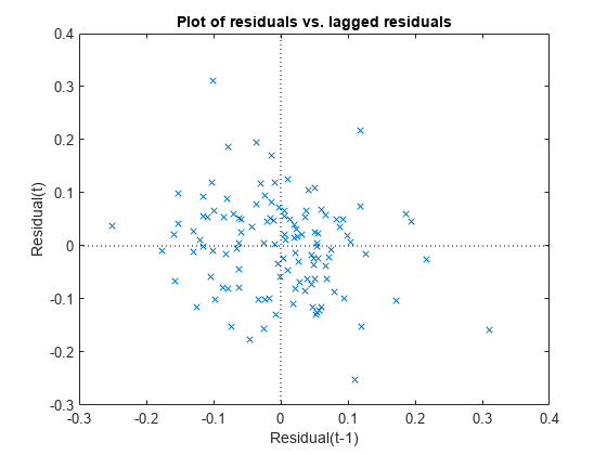

Figure contains an axes object. The axes object with title Plot of residuals vs. lagged residuals, xlabel Residual(t-1), ylabel Residual(t) contains 3 objects of type line. One or more of the lines displays its values using only markers

There is no obvious pattern in the graph. The residuals do not appear to be correlated.

plotResiduals

Syntax

Description

Input Arguments

lme — Linear mixed-effects model LinearMixedModel object

plottype — Type of residual plot 'histogram' (default) | 'caseorder' | 'fitted' | 'lagged' | 'probability' | 'symmetry'

Name-Value Arguments

ResidualType — Residual type 'Raw' (default) | 'Pearson' | 'Standardized'

Output Arguments

h — Handle to residual plot handle

Examples

Examine Residuals

See Also

`lme` — Linear mixed-effects model
`LinearMixedModel` object

`plottype` — Type of residual plot
`'histogram'` (default) | `'caseorder'` | `'fitted'` | `'lagged'` | `'probability'` | `'symmetry'`

`ResidualType` — Residual type
`'Raw'` (default) | `'Pearson'` | `'Standardized'`

`h` — Handle to residual plot
handle