Multiple-Edge Response (MER) for AMI Fast Time-Domain Nonlinear System Simulation
This example illustrates how to apply time-domain AMI equalization to a MER representation of a non-LTI (linear and time invariant) system.
This example shows how to:
Generate user defined data pattern waveforms for nonlinear systems which have been characterized with MER.
Process these nonlinear waveforms with a Tx AMI model and Rx AMI model to apply equalization.
Control the parameters of the AMI models with MATLAB commands.
Form the eye diagrams of the unequalized and equalized waveforms.
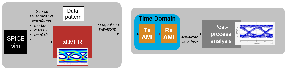
An overview of the example is illustrated below:
IBIS-AMI Overview
IBIS-AMI models and simulators are key tools for signal-integrity analysis of high-speed I/O links. The IBIS portion provides a portable, standardized description of the transmitter and receiver buffer analog behavior, while the AMI portion captures algorithmic processing such as equalization and clock/data recovery under a set of assumptions that enable efficient time-domain simulation and statistical BER estimation [1,2]. In an IBIS-AMI link, the analog path is formed by the IBIS Tx model, the channel, and the IBIS Rx model; the AMI models then apply transmitter and receiver signal processing.
In this example, the MER analysis uses a SPICE behavioral model in Parallel Link Designer to characterize the nonlinear analog response of the channel, allowing complex pull-up/pull-down behavior at the transmitter to illustrate the value of MER-based analysis. The AMI System object is used to include linear transmitter equalization and nonlinear receiver equalization within the overall simulation flow.
A key assumption in this MER workflow is that the transmitter equalization is linear time-invariant (LTI). Therefore, first determine the nonlinear analog response in isolation using the MER representation, then apply the transmitter equalization, followed by the receiver equalization. This ordering is acceptable here because LTI blocks can be reordered without changing the overall response; however, the assumption would not hold for self-adaptive or nonlinear transmitter equalization (for example, an adaptive transmitter FFE).
Use MER to Generate Accurate Nonlinear System Waveforms
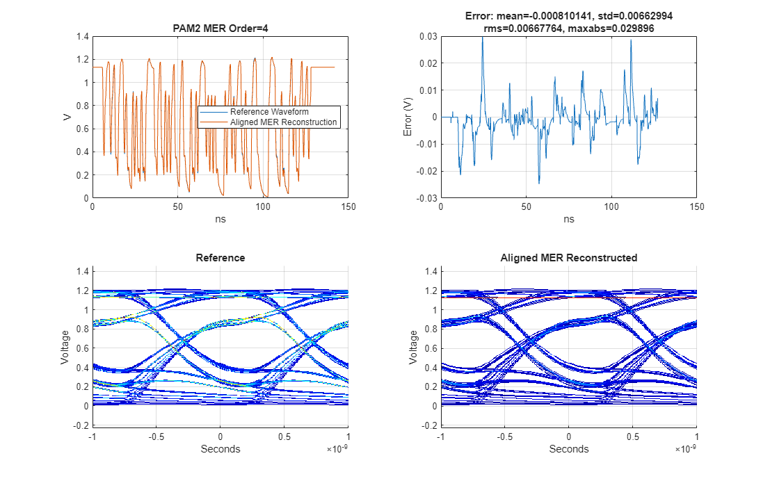
As illustrated in Using Multiple-Edge Response (MER) to Represent Nonlinear Systems, MER can be used to generate accurate nonlinear system waveforms. For our study, these waveforms are the analog model composed of the linear channel, non-LTI transmitter and transparent receiver. Later AMI processing will apply the linear transmitter equalization and nonlinear receiver equalization. This particular system required MER of order 4 to yield accurate representation. The following MATLAB code reads in the source waveforms from a Parallel Link Designer project and creates the MER representation of the analog channel model.
% Define order
Order = 4;

% Define number of symbols in simulation
numSimulationUI = 2000;

% Define PRBS order of the stimulus waveform
prbsOrder = 31;

% Define samples per symbol
SamplesPerSymbol = 16;

% Define modulation. Must match modulation of Spice source waveforms.
Modulation = 2;

% Define AMI blocksize
blockSize = SamplesPerSymbol*64;

% Define ignore time for eye diagram creation.
ignoreUI = numSimulationUI/2;

% Define path to PLD project
ProjectPLD = fullfile(pwd,'MERExamplePLD');

% Define PLD sheet name
sheetname = sprintf('merlin2_order%i',Order);

% Extract PLD data and prepare for AMI simulations.  If the PLD project
% MERExamplePLD doesn't exist yet, then it will be downloaded from the Kit
% repository and simulated.
simData = spice2mer(ProjectPLD, sheetname, Order, SamplesPerSymbol);

% Get source waveforms
SourceWavesPattern = simData.PatternMat;
SourceWaves = simData.PatternWave;
SampleInterval = simData.SampleInterval;
SymbolTime = simData.SymbolTime;

% Create MER representation
TDMER = si.MER(...
    'Order', Order,...
    'Modulation', Modulation,...
    'SamplesPerSymbol', SamplesPerSymbol,...
    'PlotAxis', 'Seconds',...
    'SymbolTime', SymbolTime,...
    'Specification', 'Wave',...
    'SourceWaves', SourceWaves,...
    'SourceWavesPattern', SourceWavesPattern,...
    'ReferenceWave',simData.ReferenceWave,...
    'ReferenceWavePattern',simData.ReferencePattern);

% Visualize the accuracy of MER representation
h2 = figure('IntegerHandle','off');
plotValidation(TDMER)
set(h2,'Units','normalized','Position',[ 0 0 1 1]);
Calculate Voltage Reference
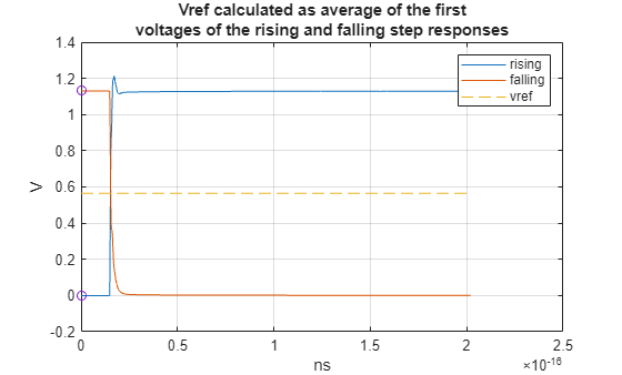
This single-ended system nominally ranges between 0 and 1.2 Volts, but the AMI model utilized is a generic SerDes model. The sampler inside the DFE assumes the input is a differential signal with a voltage reference of 0 Volts. Therefore, calculate the voltage reference, vref, from the average of the first voltages of the simple rising- and falling-step responses. Before processing with the AMI model, vref will be subtracted out to shift the signal to swing around 0 Volts, later when processing the equalized waveform, vref will be added back. This will ensure that the voltage reference voltage is maintained after the waveform conditioning.
% Calculate voltage reference from the average of the starting and ending
% voltage of the rising and falling step responses.
riseNdx = SourceWavesPattern(:,end)==1 & all(SourceWavesPattern(:,1:end-1)==0,2);
fallNdx = SourceWavesPattern(:,end)==0 & all(SourceWavesPattern(:,1:end-1)==1,2);
riseAndFallWave = SourceWaves(:,riseNdx|fallNdx);
vref = mean(riseAndFallWave(1,:));

figure('IntegerHandle','off');
plot(simData.Time*1e-9,riseAndFallWave,[simData.Time(1),simData.Time(end)]*1e-9,vref*[1 1],'--',...
[simData.Time(1),NaN,simData.Time(1)]*1e-9,[riseAndFallWave(1,1),NaN,riseAndFallWave(1,2)],'o')
grid on
legend('rising','falling','vref')
xlabel('ns')
ylabel('V')
title(sprintf('Vref calculated as average of the first\nvoltages of the rising and falling step responses'))
The validation plot shows that the MER of order 4 has a max absolute error of about 30 mV. The maximum absolute error for MER orders 1 through 6 are 421 mV, 153 mV, 68 mV, 30 mV, 15.5 mV and 15.15 mV. The choice of utilizing order 4 balances accuracy and complexity sufficient for the example study.
Set Up Transmitter AMI System
When IBIS-AMI models are used in modern simulators like Serial Link Designer, they are set up and configured automatically. But here, manually configure the transmitter AMI models for use with the SerDes Toolbox serdes.AMI system object. This transmitter AMI model contains a single feed-forward equalizer (FFE) with one pre-cursor tap and three post-cursor taps. The equalizer is not adaptive, and the mode can either be fixed or off (by-pass mode). The FFE taps values are set so the first post-cursor tap has a 5% weight. This setting was determined to balance the total equalization between the transmitter and receiver capabilities.
The serdes.AMI system object allows for low level interaction with the AMI model through the input string. A helper function, ParameterAMI, is utilized to define the adapt and fixed modes of the model, set parameters and finally create the AMI input string.
The transmitter AMI model itself was created with the SerDes toolbox SerDes designer app and Simulink.
% Define the root name
amiRootName = 'simple_serdes';

% Create Tx AMI object
txAMI1 = serdes.AMI;

% Define library name and path
txAMI1.LibraryName = [amiRootName,'_tx_',computer('arch')];
txAMI1.LibraryPath = pwd;
txAMIfilename = [amiRootName,'_tx.ami'];

% Declare the model as GetWave capable
txAMI1.InitOnly = false;

% Define symbol time and sample interval
txAMI1.SymbolTime = SymbolTime;
txAMI1.SampleInterval = SampleInterval;

% Define row size for the length of the impulse response
rowSize = 1000;
txAMI1.RowSize = rowSize;

% Define the blocksize for the GetWave simulation
txAMI1.BlockSize = blockSize;

% Define how the model behaves in adapt and fixed mode. This transmitter
% model doesn't adapt, so the adapt mode is the same as fixed.
ModeIndices = 1;
AdaptModeIndex = 1;
FixedModeIndex = 1;
txParameters = ParameterAMI(txAMIfilename,ModeIndices,AdaptModeIndex,FixedModeIndex);
Summary of mode settings for analysis:
FFE.Mode: Adapt: 1/ fixed, Fixed: 1/ fixed
% Display all parameters
DisplayParameters(txParameters)
All In and InOut AMI Parameters for simple_serdes_tx.ami: 1 FFE.Mode List_Tip (Value:String)| 1:fixed 0:off 2 FFE.TapWeights.m1 3 FFE.TapWeights.p0 4 FFE.TapWeights.p1 5 FFE.TapWeights.p2 6 FFE.TapWeights.p3
% Set Tx Equalization. One pre-cursor tap and three post-cursor taps
ffetaps = [0, 0.95, -0.05,0 0];
txParameters.SetParameter('FFE.TapWeights.m1',ffetaps(1));
txParameters.SetParameter('FFE.TapWeights.p0',ffetaps(2));
txParameters.SetParameter('FFE.TapWeights.p1',ffetaps(3));
txParameters.SetParameter('FFE.TapWeights.p2',ffetaps(4));
txParameters.SetParameter('FFE.TapWeights.p3',ffetaps(5));

% Set fixed mode behavior
txInputString = FixedInputString(txParameters);
txAMI1.InputString = txInputString;
Set Up Receiver AMI System
The receiver AMI model contains a combined four-tap decision-feedback equalizer (DFE) and clock and data recovery (CDR) block. The receiver model itself was created with the SerDes toolbox SerDes designer app and Simulink.
% Create Rx AMI object
rxAMI1 = serdes.AMI;

% Define library name and path
rxAMI1.LibraryName = [amiRootName,'_rx_',computer('arch')];
rxAMI1.LibraryPath = pwd;
rxAMIfilename = [amiRootName,'_rx.ami'];

% Define symbol time and sample interval.
rxAMI1.SymbolTime = SymbolTime;
rxAMI1.SampleInterval = SampleInterval;

% Define row size for the length of the impulse response
rxAMI1.RowSize = rowSize;

% Define blocksize for GetWave simulation
rxAMI1.BlockSize = blockSize;

% Declare model as GetWave capable
rxAMI1.InitOnly = false;

% Define how the model behaves in adapt and fixed mode. From the display of
% the parameters, you can identify the indices of the mode, and the
% indices of the List_Tip members. ParameterAMI with only one input
% argument will provide an interactive way of determining the mode indices
% and fixed/adapt settings.
ModeIndices = 1;    % DFECDR.Mode is the first parameter
AdaptModeIndex = 1; % Adapt is the first in the list
FixedModeIndex = 3; % Fixed is the third in the list
rxParameters = ParameterAMI(rxAMIfilename,ModeIndices,AdaptModeIndex,FixedModeIndex);
Summary of mode settings for analysis:
DFECDR.Mode: Adapt: 2/ adapt, Fixed: 1/ fixed
% Display all parameters and List_Tip members
DisplayParameters(rxParameters)
All In and InOut AMI Parameters for simple_serdes_rx.ami: 1 DFECDR.Mode List_Tip (Value:String)| 2:adapt 0:off 1:fixed 2 DFECDR.Phase 3 DFECDR.PhaseOffset 4 DFECDR.ReferenceOffset 5 DFECDR.TapWeights.p1 6 DFECDR.TapWeights.p2 7 DFECDR.TapWeights.p3 8 DFECDR.TapWeights.p4
Define Data pattern and Generate Unequalized Waveform
Determine the data pattern for the simulations from the declared PRBS order and the number of unit intervals (UI) to run. Here, utilize the MER representation to create an accurate waveform to model the nonlinear behavior of the analog channel of the system.
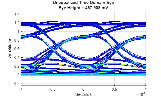
Visualize the waveform with an eye diagram and quantify the eye height at time=0 so as to quantify the impact of the equalization on eye height.
% Generate data pattern
dataPattern = prbs(prbsOrder,numSimulationUI);

% Generate unequalized waveform
TimeDomainWaveUnEQ = makeWave(TDMER,dataPattern);

% Visualize unequalized waveform with eye diagram
UnEqualizedEyeObj1 = eyeDiagramSI(...
    'SymbolTime',SymbolTime,...
    'SampleInterval',SampleInterval,...
    'Modulation',Modulation,...
    'SymbolThresholds',vref);

UnEqualizedEyeObj1(TimeDomainWaveUnEQ(ignoreUI*SamplesPerSymbol:end))

figure('IntegerHandle','off');
plot(UnEqualizedEyeObj1), grid on, colorbar off
uneqmsg = sprintf('Unequalized Time Domain Eye\nEye Height = %g mV',UnEqualizedEyeObj1.eyeHeight*1e3);
title(uneqmsg)
Set Up Impulse Response
This example does not utilize Init analysis to initialize the equalization but the IBIS-AMI standard require AMI_Init to be run before AMI_GetWave, so create a dummy impulse response to use. See Multiple-Edge Response (MER) for AMI Statistical Nonlinear System Analysis for more information about Init analysis.
% Dummy impulse response
initImpulse = zeros(rowSize,1);
initImpulse(SamplesPerSymbol*2+1) = 1/SampleInterval;
Experiment Setup and Simulation
For this study, use three different sets of DFE tap values, with the DFE in "fixed" mode, to understand their impact on the nonlinear system behavior. These three sets are defined below by the rows of the matrix caseDFETaps. The following code loops through the three cases, sets the DFE taps, sets up the receiver AMI model in fixed mode and processes the input waveform one blocksize length chunk at a time. The resulting waveforms are stored in the columns of rxTimeDomainWaveEQ. To understand better the adaptive behavior of the model, see the section "Appendix A: Observing adaptive behavior".
% DFE taps for cases 1, 2 and 3
caseDFETaps = [-0.24262   0.033522  0.044833  0.010116;
    -0.105414 -0.099997 -0.046691 -0.020842;
    -0.17402  -0.033238 -0.000929 -0.005363];

% Determine length of total simulation and initialize output vector
tdlen = floor(length(TimeDomainWaveUnEQ)/blockSize)*blockSize;
rxTimeDomainWaveEQ = zeros(tdlen,size(caseDFETaps,1));

% Loop over DFE tap cases
for jj = 1:size(caseDFETaps,1)

    % Set in/out parameters
    rxParameters.SetParameter('DFECDR.TapWeights.p1',caseDFETaps(jj,1));
    rxParameters.SetParameter('DFECDR.TapWeights.p2',caseDFETaps(jj,2));
    rxParameters.SetParameter('DFECDR.TapWeights.p3',caseDFETaps(jj,3));
    rxParameters.SetParameter('DFECDR.TapWeights.p4',caseDFETaps(jj,4));

    % Get fixed mode AMI input string
    rxInputString = FixedInputString(rxParameters);
    rxAMI1.InputString = rxInputString;

    % Time Domain AMI simulation. Process a blocksize length of waveform at
    % a time.
    txTimeDomainWaveEQ = zeros(tdlen,1);
    ClockIn = -1;
    for ii = 1:floor(length(TimeDomainWaveUnEQ)/blockSize)
        ndx = (ii-1)*blockSize+1:ii*blockSize;
        [txTimeDomainWaveEQ(ndx),txImpulseOutDummy] = txAMI1(TimeDomainWaveUnEQ(ndx)-vref, initImpulse, ClockIn);
        [rxTimeDomainWaveEQ(ndx,jj),~] = rxAMI1(txTimeDomainWaveEQ(ndx), txImpulseOutDummy, ClockIn);
    end

    txAMI1.release;
    rxAMI1.release;
end
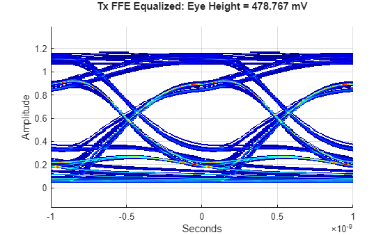
Tx Equalization-Only Response
The impact of the transmitter FFE on the system performance is quantified below.
% Visualize Tx equalized only waveform with eye diagram
TxOutEyeObj = eyeDiagramSI(...
    'SymbolTime',SymbolTime,...
    'SampleInterval',SampleInterval,...
    'Modulation',Modulation,...
    'SymbolThresholds',vref);

% Process transmitter equalized waveform with eye object
TxOutEyeObj(txTimeDomainWaveEQ(ignoreUI*SamplesPerSymbol:end)+vref)

% Visualize eye
figure('IntegerHandle','off');
plot(TxOutEyeObj), grid on, colorbar off
title(sprintf('Tx FFE Equalized: Eye Height = %g mV\n',TxOutEyeObj.eyeHeight*1e3));
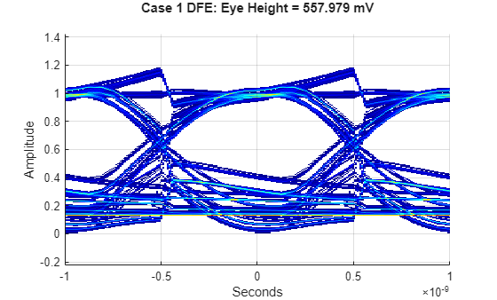
DFE Equalization Case 1
The first set of DFE taps are obtained from a Statistical analysis of the impulse response derived from the rising step response. As can be seen in the eye diagram below, the voltages around the upper symbol are well equalized but the lower symbol voltages are scattered. From this experiment it is clear that determining an optimal set of DFE taps may be difficult.
caseColumn = 1;

EqualizedEyeObj1 = eyeDiagramSI(...
    'SymbolTime',SymbolTime,...
    'SampleInterval',SampleInterval,...
    'Modulation',Modulation,...
    'SymbolThresholds',vref);

EqualizedEyeObj1(rxTimeDomainWaveEQ(ignoreUI*SamplesPerSymbol:end,caseColumn)+vref)

figure('IntegerHandle','off');
plot(EqualizedEyeObj1), grid on, colorbar off
title(sprintf('Case 1 DFE: Eye Height = %g mV\n',EqualizedEyeObj1.eyeHeight*1e3));
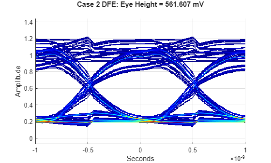
DFE Equalization Case 2
The second set of DFE taps are obtained from a Statistical analysis of the impulse response derived from the falling step response. As can be seen in the eye diagram below, the voltages around the lower symbol are well equalized but the upper symbol voltages are all over the place. From this experiment, you can conclude that different sets of DFE taps can optimize different symbol levels of the equalized waveform.
caseColumn = 2;

EqualizedEyeObj2 = eyeDiagramSI(...
    'SymbolTime',SymbolTime,...
    'SampleInterval',SampleInterval,...
    'Modulation',Modulation,...
    'SymbolThresholds',vref);

EqualizedEyeObj2(rxTimeDomainWaveEQ(ignoreUI*SamplesPerSymbol:end,caseColumn)+vref)

figure('IntegerHandle','off');
plot(EqualizedEyeObj2), grid on, colorbar off
title(sprintf('Case 2 DFE: Eye Height = %g mV\n',EqualizedEyeObj2.eyeHeight*1e3));
DFE Equalization Case 3
The third set of DFE taps are obtained from averaging together the case 1 and 2 tap values and results in a significantly larger eye height. From this experiment, you can conclude that better methods of determining DFE tap values are needed, perhaps even new DFE equalizer circuits that can take advantage of the known symbol asymmetry to better optimize system performance [3].
caseColumn = 3;

EqualizedEyeObj3 = eyeDiagramSI(...
    'SymbolTime',SymbolTime,...
    'SampleInterval',SampleInterval,...
    'Modulation',Modulation,...
    'SymbolThresholds',vref);

EqualizedEyeObj3(rxTimeDomainWaveEQ(ignoreUI*SamplesPerSymbol:end,caseColumn)+vref)

figure('IntegerHandle','off');
plot(EqualizedEyeObj3), grid on, colorbar off
title(sprintf('Case 3 DFE: Eye Height = %g mV\n',EqualizedEyeObj3.eyeHeight*1e3));
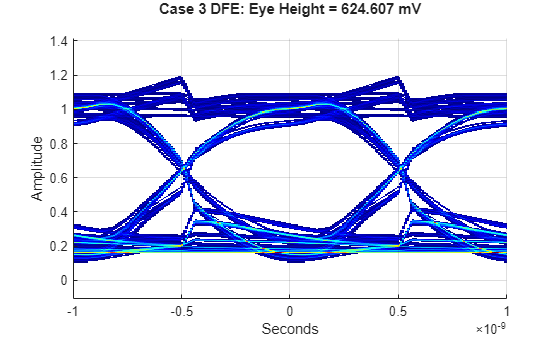
The above three DFE cases show the impact of the DFE on the upper and lower parts of the eye diagram. While case 3, with the average of case 1 and case 2 DFE taps, yields the largest eye opening, it isn't entirely evident if these DFE taps are optimal or not. More work is required to design DFE adaptation algorithms for these types of nonlinear systems.
Conclusion
This example illustrates how to utilize MER representation and AMI models to simulate and analyze a nonlinear system in the time domain with equalization. This example illustrates how to generate nonlinear waveforms with the si.MER class, how to configure and run AMI models in MATLAB and visualize the resulting waveforms with eyeDiagramSI. This approach allows the user to simulate any NRZ data pattern desired and is much faster than a dedicated SPICE simulation.
Explore these concepts further by:
Applying MER methodology to your own AMI models
Learning about DFE algorithms that apply different voltage tap correction dependent on the polarity of the prior transitions [3].
Modifying "Appendix A: Observing adaptive behavior" to initialize the experiment with the impulse response from the falling step response.
Appendix A: Observing adaptive behavior
The above time domain GetWave simulations are run with the DFE in the fixed mode, where the DFE taps are fixed to an initial value and not adapted with the DFE block's adaptive engine. The appendix illustrates how to run the receiver in adapt mode and observe how the output AMI parameters change over time. One of the key abilities of an AMI model is the ability to run Init (for impulse based analysis) and GetWave together, yielding superior capabilities to either Init or GetWave run in isolation. For the example DFE, in adapt mode, the DFE taps estimated from the impulse response are used as the initial DFE taps in GetWave. This allows the more accurate but slower running GetWave simulation to begin the DFE tap adaptation nearer the optimal tap values.
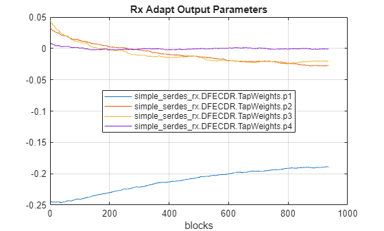
As illustrated above, the DFE taps obtained from Init with an impulse derived from the rising or falling step responses do not result in the best tap values. The following code shows that when the model is run in "adapt" mode the DFE tap values converge near to the case 3 DFE tap values and yields similar eye height values.
% Get impulse response from the rising step response
ImpulseUnEQ =  step2impulse(SourceWaves(:,riseNdx),SampleInterval);

% Impulse response from the falling step response
% ImpulseUnEQ = -step2impulse(SourceWaves(:,fallNdx),SampleInterval);

% Define number of symbols in simulation
numSimulationUI2 = 60000;

% Generate data pattern
dataPattern2 = prbs(prbsOrder,numSimulationUI2);

% Generate unequalized waveform
TimeDomainWaveUnEQ2 = makeWave(TDMER,dataPattern2);

% Determine length of total simulation and initialize output vector
tdlen2 = floor(length(TimeDomainWaveUnEQ2)/blockSize)*blockSize;
rxTimeDomainWaveEQ2 = zeros(tdlen2,1);

% Setup the receiver in adaptive mode
rxInputString = AdaptInputString(rxParameters);
rxAMI1.InputString = rxInputString;

% Time Domain AMI simulation. Process a blocksize length of waveform at a time.
ClockIn = -1;
for ii = 1:floor(length(TimeDomainWaveUnEQ2)/blockSize)
    ndx = (ii-1)*blockSize+1:ii*blockSize;
    [txTimeDomainWaveEQ2,initImpulseTmp] = txAMI1(TimeDomainWaveUnEQ2(ndx)-vref, ImpulseUnEQ, ClockIn);
    rxTimeDomainWaveEQ2(ndx) = rxAMI1(txTimeDomainWaveEQ2, initImpulseTmp, ClockIn);
end

% Release AMI blocks to finalize the output parameters
txAMI1.release;
rxAMI1.release;

% Process output AMI parameter strings
TDOutputParams = rxAMI1.AMIData.GetWaveAMIOutput;
ReadTDOutputString(rxParameters,TDOutputParams);

% Select the output DFE tap parameters (exclude the output CDR phase waveform)
parameterSelect = 2:5;

% Visualize tap values
figure('IntegerHandle','off');
plot(rxParameters.TDOutputValues(:,parameterSelect));
hLeg = legend(rxParameters.TDOutputNames(parameterSelect),'location','best','interpreter','none');
hLeg.ItemHitFcn = @si.MER.ToggleLineVisibility;
title(sprintf('Rx Adapt Output Parameters'));
xlabel('blocks')
grid on
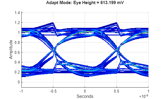
Create an eye diagram with the same number of unit intervals as the above eye diagrams for a fair comparison. Comparing this eye height to the eye height from case 3 above shows very similar performance.
AdaptEqualizedEyeObj = eyeDiagramSI(...
    'SymbolTime',SymbolTime,...
    'SampleInterval',SampleInterval,...
    'Modulation',Modulation,...
    'SymbolThresholds',vref);

% Number of unit intervals that the other eye diagrams used
nUI = numSimulationUI - ignoreUI;

AdaptEqualizedEyeObj(rxTimeDomainWaveEQ2(end-nUI*SamplesPerSymbol:end)+vref)

figure('IntegerHandle','off')
plot(AdaptEqualizedEyeObj), grid on, colorbar off
title(sprintf('Adapt Mode: Eye Height = %g mV\n',AdaptEqualizedEyeObj.eyeHeight*1e3));
The initial adaptive DFE tap values are very similar to the case 1 DFE taps values.
disp(rxParameters.TDOutputValues(1,parameterSelect))
-0.2435 0.0325 0.0438 0.0092
The last adaptive DFE tap values are very similar to the case 3 DFE tap values.
disp(rxParameters.TDOutputValues(end,parameterSelect))
-0.1887 -0.0271 -0.0200 -0.0009
References
[1] Chae, Joo-Hyung, Minchang Kim, Sungphil Choi, and Suhwan Kim. A 10.4-Gb/s 1-Tap Decision Feedback Equalizer With Different Pull-Up and Pull-Down Tap Weights for Asymmetric Memory Interfaces. IEEE Transactions on Circuits and Systems II: Express Briefs 67, no. 2 (2020): 220–24. https://doi.org/10.1109/TCSII.2019.2911017.