CVT with Custom Belt Pulley Components
R2026bThis example shows how to use a custom belt pulley library to build a pulley-based continuously variable transmission (CVT). The CVT comprises two variable-radius pulleys connected by a closed-loop belt. The custom domain accounts for changes in pulley radius and the effects on belt tension and belt mass distribution. The input pulley increases its radius with speed via centrifugal force, while the output pulley adjusts its radius based on belt tension and a spring. An external source applies torque to the input pulley, and the belt transmits power to the output pulley. The distance between the input and output pulleys is 200 mm, and the radius of each pulley can vary from 22 mm to 43 mm.
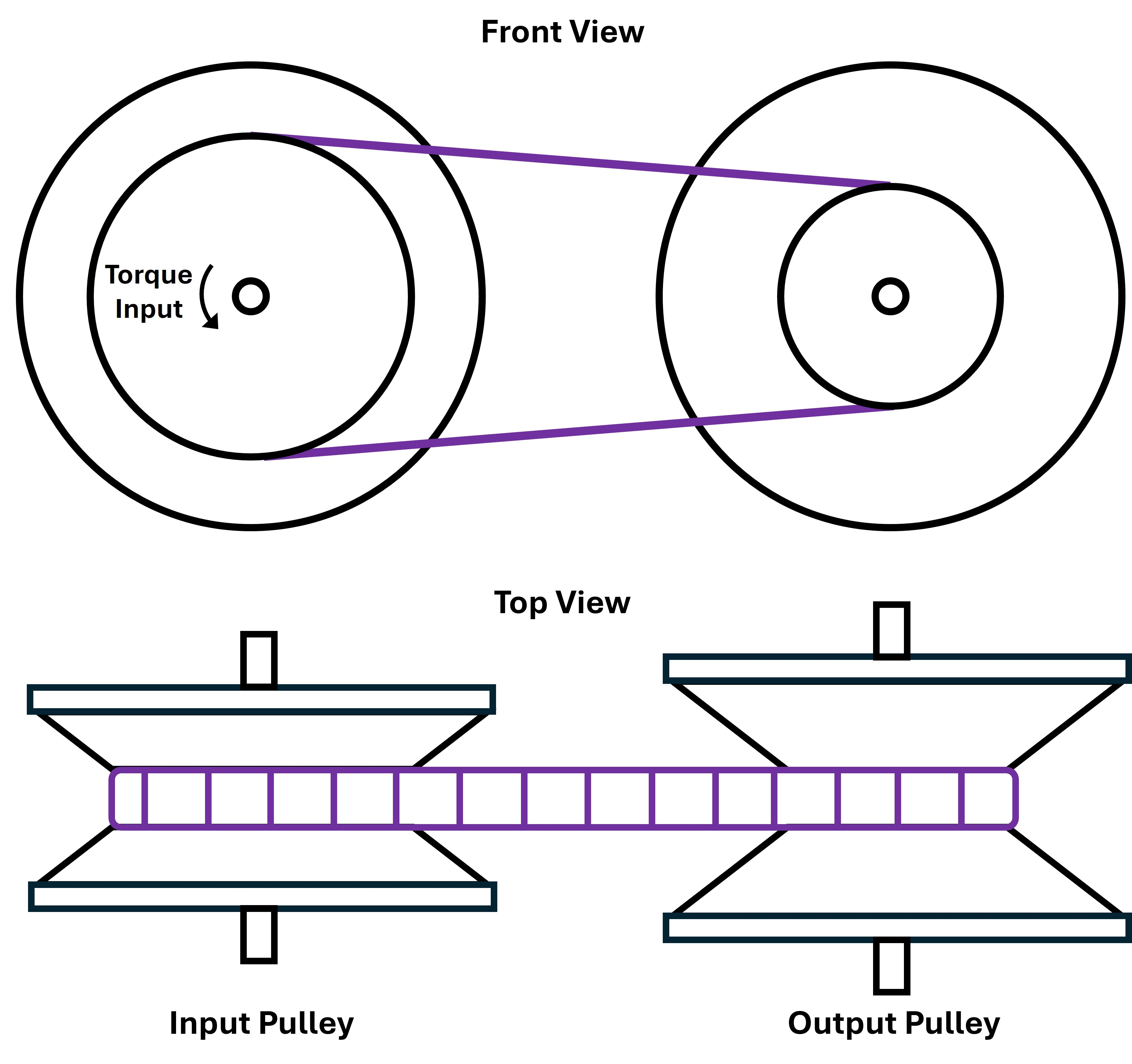
Configure CVT Model
The model represents a typical scooter CVT and consists of three parts: a belt drive network using the custom library, a subsystem for the input pulley radius dynamics, and another subsystem for the output pulley radius dynamics. Open the model.
open_system('CustomBeltPulleyLibraryCVT');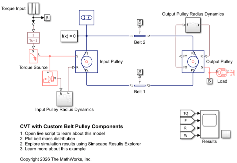
The custom Belt Pulley (BP) library contains four blocks: Belt (BP), Belt (BP-PB), Belt Pulley Properties (BP), and Pulley (BP). A Belt (BP) block provides the connection between two Pulley (BP) blocks. A Belt (BP-PB) block serves as an interface between a Pulley (BP) block and a position-based mechanical translational network. A Belt Pulley Properties (BP) block specifies the domain parameters of the network.
open_system('belt_pulley_lib');
Specify Pulley Radius
The Pulley (BP) block receives the pulley radius through the physical signal input port R. Select Input pulley radius to enable the port.
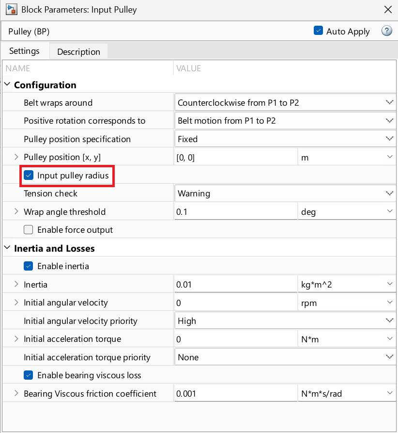
To enable the ports programmatically, enter:
set_param('CustomBeltPulleyLibraryCVT/Input Pulley','input_radius','true');
set_param('CustomBeltPulleyLibraryCVT/Output Pulley','input_radius','true');
Review Radius Dynamics Subsystem
Centrifugal weights in the input pulley force the cone-shaped plates apart, while the spring in the output pulley pushes the cone-shaped plates together against belt tension. The example uses simple tabular models for the dynamics of the radii. You can replace these lookup tables with higher-fidelity physics models.
The Input Pulley Radius Dynamics subsystem uses a lookup table to calculate the radius from the pulley rotational speed. Open the Input Pulley Radius Dynamics subsystem.
open_system('CustomBeltPulleyLibraryCVT/Input Pulley Radius Dynamics');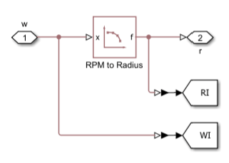
The Output Pulley Radius Dynamics subsystem uses a lookup table to determine the radius from the force that the belt segments exert on the shaft. Open the Output Pulley Radius Dynamics subsystem.
open_system('CustomBeltPulleyLibraryCVT/Output Pulley Radius Dynamics');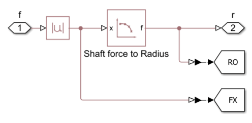
Analyze Results
The model simulates the scenario according to the simulation time, t.
t = 0.0 - 1.0 s — The system is at rest with no input torque.
t = 1.0 - 2.0 s — The input torque ramps linearly and saturates to 5 N*m at t = 2.0 s.
t = 2.0 - 10.0 s — The pulleys accelerate toward steady state. The gear ratio changes continuously.
All Simscape blocks are in static equilibrium at t = 0.0 s. The table shows the high priority initial targets that the model uses.
Block | Initial Target | Value |
| Angular velocity |
|
| Angular velocity |
|
| Belt tension |
|
| Belt tension |
|
Since the belt tensions are the same at t = 0.0 s, the initial net torque to each of the pulleys is zero.
To view the results, enter:
open_system('CustomBeltPulleyLibraryCVT/Results');
sim('CustomBeltPulleyLibraryCVT');
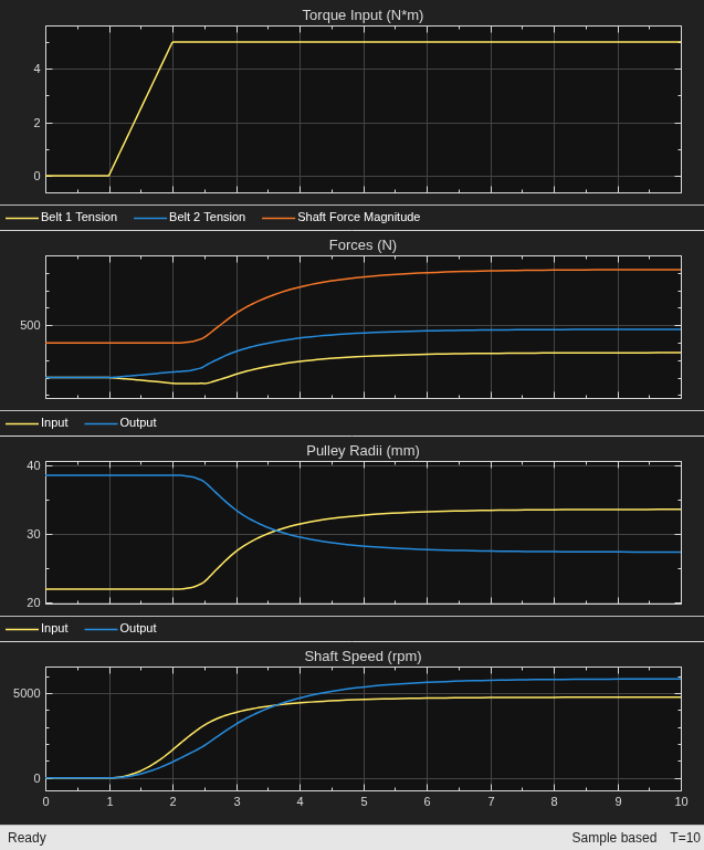
Initially, all components are at rest, with the input pulley radius smaller than the output pulley radius. After t = 1.0 s, the input pulley accelerates, causing its radius to increase as speed rises. At the same time, the increasing shaft force magnitude reduces the output pulley radius. Between t = 3.0 s and t = 4.0 s, the gear ratio reverses. The system then reaches steady state with the output pulley speed near 6000 rpm.
Plot the belt mass distribution across the belt drive.
CustomBeltPulleyLibraryCVTPlot1
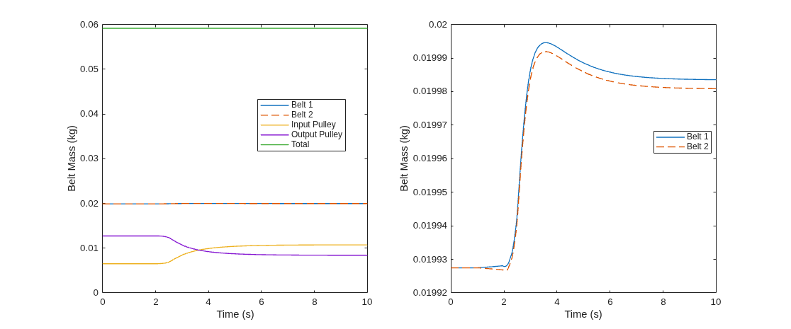
The left figure shows the belt mass distribution over time. The belt gradually moves from occupying more of the output pulley to more of the input pulley. The system conserves total belt mass throughout the simulation. The right figure shows the mass variations of the belt segments.

