Simulate and Visualize Land Mobile-Satellite Channel
This example shows how to model a two-state land mobile-satellite (LMS) channel model by generating a state series, its respective space series, and the channel coefficients. In a scenario involving a satellite terminal and a mobile terminal, a signal being transmitted through the channel does not always have an ideal line-of-sight path. In some cases, the signal experiences phenomena such as Doppler shift, shadowing, and multipath fading. Appropriately modeling the effects of such phenomena is essential to properly design end-to-end communication links that are able to handle and compensate the effects of the channel.
Introduction
An LMS channel model is used to simulate the channel envelope that is observed in a satellite-to-ground channel. Given the moving nature of the terminals, the channel envelope experiences variations due to movement of the transmitting and receiving terminals, blockage due to buildings and foliage, shadowing, and multipath.
This example models ITU-R P.681-11 LMS channel and Lutz LMS channel by using a two-state semi-Markov chain, where the channel alternates between a good and bad state. A good state is characterized by either line-of-sight conditions or partial shadowing conditions, whereas a bad state is characterized by either severe shadowing conditions or complete blockage. Both the channel models are used for a single geostationary satellite. An ITU-R P.681-11 LMS channel uses Loo distribution in both good and bad state, whereas Lutz LMS channel uses Rician distribution in good state and Rayleigh with log-normal distribution in bad state. The data sets provided for ITU-R P.681-11 channel in [1] are applicable for frequency range of 1.5 GHz to 20 GHz, and the data set provided for Lutz LMS channel in [2] is applicable for frequency of 1.54 GHz (L-band).
The following block diagram shows the procedure to model the LMS channel:
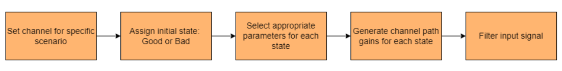
Channel Setup
Set up a channel between a satellite terminal and a mobile terminal on the ground using either p681LMSChannel or lutzLMSChannel System object.
Set these parameters to model a specific scenario using ITU-R P.681-11 LMS channel:
Environment
Carrier frequency
Elevation angle
Speed of the ground terminal
Azimuth orientation of the ground terminal
Set these parameters to model a specific scenario using Lutz LMS channel:
Rician K-factor
Lognormal fading parameters
State duration distribution
Mean state duration
Maximum Doppler shift
In addition to a specific scenario modeling, the LMS channel requires defining these parameters:
Sampling rate of input signal
Initial state of the channel
Fading technique
By default, the example selects an ITU-R P.681-11 LMS channel and configures the channel to an urban scenario with 3.8 GHz carrier frequency having a mobile terminal moving at a speed of 2 m/s.
% Create an ITU-R P.681-11 channel or Lutz LMS channel chan =p681LMSChannel; % Set channel properties if isa(chan,"p681LMSChannel") % For ITU-R P.681 LMS channel % Environment type chan.Environment = "Urban"; % Carrier frequency (in Hz) chan.CarrierFrequency = 3.8e9; % Elevation angle with respect to ground plane (in degrees) chan.ElevationAngle = 45; % Speed of movement of ground terminal (in m/s) chan.MobileSpeed = 2; % Direction of movement of ground terminal (in degrees) chan.AzimuthOrientation = 0; else % For Lutz LMS channel % Rician K-factor (in dB) chan.KFactor = 5.5; % Lognormal fading parameters (in dB) chan.LogNormalFading = [-13.6 3.8]; % State duration distribution chan.StateDurationDistribution =
"Exponential"; % Mean state duration (in seconds) chan.MeanStateDuration = [21 24.5]; % Maximum Doppler shift (in Hz) chan.MaximumDopplerShift = 2.8538; end % Sampling rate (in Hz) chan.SampleRate = 400;
Assign a suitable initial state for the channel.
chan.InitialState =  "Good";
Set the fading technique used to realize the Doppler spectrum. The fading technique is either "Filtered Gaussian noise" or "Sum of sinusoids". When FadingTechnique property is set to "Sum of sinusoids", you can also set the number of sinusoids through NumSinusoids property.
chan.FadingTechnique = "Filtered Gaussian noise"; Initialize random number generator with seed. Vary the seed to obtain different channel realizations. The default value 73 is an arbitrary value.
seed = 73;
chan.RandomStream = "mt19937ar with seed";
chan.Seed = seed;
Display the properties of the channel.
disp(chan)
  p681LMSChannel with properties:

                NumStates: 2
               SampleRate: 400
             InitialState: "Good"
         CarrierFrequency: 3.8000e+09
           ElevationAngle: 45
              MobileSpeed: 2
       AzimuthOrientation: 0
    SatelliteDopplerShift: 0
              Environment: "Urban"
         ChannelFiltering: true

  Show all properties
Channel Model
Generate the channel for a duration of 100 seconds. Use random samples as input waveform.
% Set random number generator with seed
rng(seed);
% Channel duration (in seconds)
chanDur = 100;
% Random input waveform
numSamples = floor(chan.SampleRate*chanDur)+1;
in = complex(randn(numSamples,1),randn(numSamples,1));
% Pass the input signal through channel
[fadedWave,channelCoefficients,sampleTimes,stateSeries] = step(chan,in);
Channel Visualization
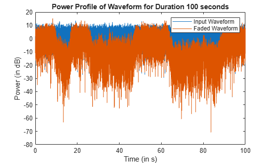
Visualize the power profile, the space series, and the state series generated as part of channel modeling.
Plot the power profile of input waveform and the faded waveform.
figure(1)
plot(sampleTimes,20*log10(abs(in)),sampleTimes,20*log10(abs(fadedWave)))
title(['Power Profile of Waveform for Duration ' num2str(chanDur) ' seconds'])
legend('Input Waveform', 'Faded Waveform')
xlabel('Time (in s)')
ylabel('Power (in dB)')
Plot the space series to show how the instantaneous power of the channel envelope varies with time.
figure(2)
plot(sampleTimes,20*log10(abs(channelCoefficients)))
title(['Space Series of Channel for Duration ' num2str(chanDur) ' seconds'])
xlabel('Time (in s)')
ylabel('Path Gain (in dB)')

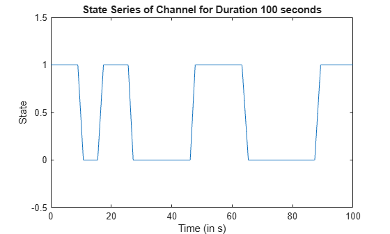
Plot the state series to show how the channel state varies with time.
figure(3)
plot(sampleTimes,stateSeries)
title(['State Series of Channel for Duration ' num2str(chanDur) ' seconds'])
axis([0 sampleTimes(end) -0.5 1.5])
xlabel('Time (in s)')
ylabel('State')
Further Exploration
This example uses either p681LMSChannel or lutzLMSChannel System object to generate the two-state LMS channel for the defined channel properties. You can modify the properties of the System object to observe the variations with respect to time in the power profile, channel coefficients, and state series. To model the ITU-R P.681 channel for different frequency bands, you can set the parameters related to any of the data tables available in ITU-R P.681-11 Recommendation Section 3.1 Annexure 2 [1]. You can also set the ITU-R P.681 LMS channel to custom environment with any other data set available. To model the Lutz LMS channel for different scenarios, you can use the data table present in [2].
References
[1] ITU-R Recommendation P.681-11 (08/2019). "Propagation data required for the design systems in the land mobile-satellite service." P Series; Radio wave propagation.
[2] E. Lutz, D. Cygan, M. Dippold, F. Dolainsky, and W. Papke, "The land mobile-satellite communication channel-recording, statistics, and channel model", IEEE Trans. Veh. Technol., vol 40, no. 2, pp. 375-386, 1991.