이 번역 페이지는 최신 내용을 담고 있지 않습니다. 최신 내용을 영문으로 보려면 여기를 클릭하십시오.
지구-우주 전파 손실
전파 환경은 위성 통신 시스템의 지구-우주 링크 설계에 상당한 영향을 미칩니다. 지구-우주 링크에 대한 전리층 영향은 1GHz 미만의 주파수에서 크게 나타납니다. 이온화되지 않은 대기의 영향은 약 1GHz 이상 및 낮은 고도각에서 중요해집니다. Recommendation ITU-R P.618[1]은 지구-우주 또는 우주-지구 방향으로 작동하는 지구-우주 시스템 계획에 필요한 전파 파라미터를 예측합니다. P.618은 강우 감쇠, 가스 감쇠, 강수 및 구름 감쇠, 대류권 신틸레이션으로 인한 감쇠 등 대류권의 영향만을 다룹니다.
경우에 따라 음성, 데이터, 텔레비전 신호를 지속적으로 고품질로 전송해야 할 수도 있습니다. 이러한 경우 p618Config 객체를 사용하여 강우 감쇠, 가스 감쇠, 구름 및 안개 감쇠, 대류권 신틸레이션으로 인한 감쇠와 같은 대류권 효과를 모델링할 수 있습니다. 그런 다음 구성 파라미터 설정을 초기화하는 p618PropagationLosses 함수를 사용하여 지구-우주 전파 손실, 교차 편파 식별, 지상국 안테나의 하늘 잡음 온도를 계산할 수 있습니다.
폭우는 지구-우주 링크에서 큰 감쇠 값을 유발합니다. 사이트 다이버시티(site diversity)를 사용하면 링크 트래픽을 대체 지구국으로 라우팅할 수 있으므로 시스템 안정성이 향상됩니다. 사이트 다이버시티 시스템은 다음 옵션 중 하나로 분류됩니다.
평형(balanced): 두 링크의 감쇠 임계값이 동일합니다.
불평형(unbalanced): 두 링크의 감쇠 임계값이 동일하지 않습니다.
두 개의 지구국이 존재하는 경우, p618SiteDiversityConfig 객체를 사용하여 강우 감쇠로 인한 중단(outage)의 확률 계산에 필요한 파라미터를 모델링할 수 있습니다. 강한 비는 지구-우주 링크에서 큰 감쇠 값을 유발할 수 있습니다. 이런 경우에는 구성 파라미터 설정을 초기화하는 p618SiteDiversityOutage 함수를 사용하여, 사이트 다이버시티를 사용한 경우에 강우 감쇠로 인한 중단 확률을 계산할 수 있습니다.
초과율과 가용도 간의 상관관계
가용도는 링크가 성립되어(closed) 있어야 하는 연평균 시간 비율입니다. 다음 방정식은 가용도와 연간 초과율 간의 상관관계를 나타냅니다.
연간 초과율(%) = 100 (%) − 가용도(%)
미리 선택된 임계값이 평균적으로 1년 동안 초과되는 시간의 비율을 연간 초과 시간 비율이라고 하며, 이는 고려 중인 전파 파라미터의 초과율 또는 중단(outage)을 나타냅니다.
아래 표는 초과율 속성 범위가 가용도 범위에 매핑되는 방식을 보여줍니다.
| 감쇠 유형 | 연간 초과율 | 가용도 |
|---|---|---|
| 가스 | [0.1, 99] | [1, 99.9] |
| 구름 | [0.1, 99] | [1, 99.9] |
| 비 | [0.001, 5] | [95, 99.999] |
| 신틸레이션 | [0.01, 50] | [50, 99.99] |
| 총계 | [0.001, 50] | [50, 99.999] |
지구-우주 전파 손실
이 예제에서는 ITU(국제전기통신연합) 문서의 디지털 지도가 포함된 MAT 파일이 필요합니다. 경로에 파일이 없는 경우 다음 명령을 실행하여 MAT 파일을 다운로드하고 압축을 풉니다.
maps = exist('maps.mat','file');
p836 = exist('p836.mat','file');
p837 = exist('p837.mat','file');
p840 = exist('p840.mat','file');
matFiles = [maps p836 p837 p840];
if ~all(matFiles)
    if ~exist('ITURDigitalMaps.tar.gz','file')
        url = 'https://www.mathworks.com/supportfiles/spc/P618/ITURDigitalMaps.tar.gz';
        websave('ITURDigitalMaps.tar.gz',url);
        untar('ITURDigitalMaps.tar.gz');
    else
        untar('ITURDigitalMaps.tar.gz');
    end
    addpath(cd);
end
이 예제에서는 지구-우주 시스템 설계를 위해 전파 손실을 파라미터화하고 계산하는 방법을 보여줍니다.
p618PropagationLosses 함수로 계산되는 전파 손실은 다음과 같습니다.
대기 가스에 의한 감쇠
강우에 의한 감쇠
강수 및 구름 감쇠
대류권 신틸레이션으로 인한 감쇠
총 대기 감쇠
지구-우주 전파 손실은 주파수, 지리적 위치, 고도각에 따라 달라지도록 모델링됩니다. 전파 조건에 따라 10° 이상의 고도각에서는 대기 가스, 강우, 구름, 대류권 신틸레이션으로 인한 감쇠만 유의미합니다.
지구-우주 전파 파라미터 구성하기
디폴트 P.618 구성 객체를 만듭니다. 속성값을 변경한 다음 객체 속성을 표시합니다.
cfg = p618Config;
cfg.Frequency = 25e9;               % Signal frequency in Hz
cfg.ElevationAngle = 45;
cfg.Latitude = 30;                  % North direction
cfg.Longitude = 120;                % East direction
cfg.TotalAnnualExceedance = 0.001;  % Time percentage of excess for the total
                                    % Attenuation per annum
cfg.AntennaEfficiency = 0.65;
disp(cfg);
  p618Config with properties:

                        Frequency: 2.5000e+10
                   ElevationAngle: 45
                         Latitude: 30
                        Longitude: 120
              GasAnnualExceedance: 1
            CloudAnnualExceedance: 1
             RainAnnualExceedance: 1
    ScintillationAnnualExceedance: 1
            TotalAnnualExceedance: 1.0000e-03
            PolarizationTiltAngle: 0
                  AntennaDiameter: 1
                AntennaEfficiency: 0.6500
가벼운 강우 시 전파 손실 계산하기
지구국 높이를 0.5km로 지정하고 시간당 1mm의 약한 강우에서의 전파 손실(pl), 교차 편파 식별(xpd), 하늘 잡음 온도(tsky)를 구합니다.
전파 손실 필드 pl은 다음 감쇠를 설명합니다.
Ag: 가스 감쇠(단위: dB)Ac: 구름 및 안개 감쇠(단위: dB)Ar: 강우 감쇠(단위: dB)As: 대류권 신틸레이션으로 인한 감쇠(단위: dB)At: 총 대기 감쇠(단위: dB)
[pl,xpd,tsky] =  p618PropagationLosses(cfg, ...
                            'StationHeight',0.5, ...
                            'WaterVaporDensity',2.8, ...
                            'TotalColumnarContent',1.4, ...
                            'RainRate',1)
pl = struct with fields:
    Ag: 1.6393
    Ac: 1.2010
    Ar: 0.0811
    As: 0.3010
    At: 6.6514
xpd = 73.1657
tsky = 214.6132
사이트 다이버시티(site diversity)를 사용한 경우 강우 감쇠로 인한 중단(outage) 가능성
이 예제에서는 ITU 문서의 디지털 지도가 포함된 MAT 파일이 필요합니다. 경로에 파일이 없는 경우 다음 명령을 실행하여 MAT 파일을 다운로드하고 압축을 풉니다.
maps = exist('maps.mat','file');
p836 = exist('p836.mat','file');
p837 = exist('p837.mat','file');
p840 = exist('p840.mat','file');
matFiles = [maps p836 p837 p840];
if ~all(matFiles)
    if ~exist('ITURDigitalMaps.tar.gz','file')
        url = 'https://www.mathworks.com/supportfiles/spc/P618/ITURDigitalMaps.tar.gz';
        websave('ITURDigitalMaps.tar.gz',url);
        untar('ITURDigitalMaps.tar.gz');
    else
        untar('ITURDigitalMaps.tar.gz');
    end
    addpath(cd);
end
이 예제에서는 사이트 다이버시티를 사용한 경우에 강우 감쇠로 인한 중단 확률을 계산하는 방법을 보여줍니다.
p618SiteDiversityOutage 함수는 불평형 시스템과 평형 시스템에 적용되며 감쇠 임계값을 초과하는 결합 확률을 계산합니다.
P.618 사이트 다이버시티 파라미터 구성하기
디폴트 P.618 사이트 다이버시티 구성 객체를 만듭니다. 속성값을 변경한 다음 객체 속성을 표시합니다.
cfgSD = p618SiteDiversityConfig;
cfgSD.Frequency = 25e9;                 % Signal frequency in Hz
cfgSD.Latitude = [30 60];               % North direction
cfgSD.Longitude = [120 150];            % East direction
cfgSD.PolarizationTiltAngle = [-90 90];
cfgSD.AttenuationThreshold =  [7 7];    % Attenuation threshold on the two links
cfgSD.SiteDistance = 50;                % Separation between the two sites
disp(cfgSD);
  p618SiteDiversityConfig with properties:

                Frequency: 2.5000e+10
           ElevationAngle: [52.4099 52.4852]
                 Latitude: [30 60]
                Longitude: [120 150]
    PolarizationTiltAngle: [-90 90]
             SiteDistance: 50
     AttenuationThreshold: [7 7]
중단 확률 계산하기
지정된 사이트 다이버시티 구성에 대해 강우 감쇠로 인한 중단 확률을 계산합니다.
outage = p618SiteDiversityOutage(cfgSD, ...
                                'RainAnnualExceedances',[0.01 0.01 0.03 0.05 0.1 0.2], ...
                                'RainProbability1',0.3, ...
                                'RainProbability2',0.4);
disp(outage);
0.0030
대기 가스로 인한 감쇠
이 예제에서는 ITU 문서의 디지털 지도가 포함된 MAT 파일이 필요합니다. 경로에 파일이 없는 경우 다음 명령을 실행하여 MAT 파일을 다운로드하고 압축을 풉니다.
maps = exist('maps.mat','file');
p836 = exist('p836.mat','file');
p837 = exist('p837.mat','file');
p840 = exist('p840.mat','file');
matFiles = [maps p836 p837 p840];
if ~all(matFiles)
    if ~exist('ITURDigitalMaps.tar.gz','file')
        url = 'https://www.mathworks.com/supportfiles/spc/P618/ITURDigitalMaps.tar.gz';
        websave('ITURDigitalMaps.tar.gz',url);
        untar('ITURDigitalMaps.tar.gz');
    else
        untar('ITURDigitalMaps.tar.gz');
    end
    addpath(cd);
end
이 예제에서는 지구-우주 시스템을 설계할 때 지정된 주파수 범위에 대한 가스 감쇠를 계산하는 방법을 보여줍니다.
가스 감쇠는 신호 주파수, 고도각, 지구국 높이, 수증기 밀도에 따라 달라지도록 모델링됩니다. 전파 조건에 따라 가스 감쇠는 10GHz 이상의 주파수에서 유의미하게 나타날 수 있고, 10GHz 미만의 주파수에서는 무시할 수 있는 수준으로 나타날 수 있습니다.
P.618 전파 파라미터 구성하기
디폴트 P.618 구성 객체를 만듭니다. 속성값을 변경한 다음 객체 속성을 표시합니다.
cfg = p618Config;
cfg.Latitude = 51.5;          % North direction
cfg.Longitude = -0.14;        % West direction
cfg.GasAnnualExceedance = 10; % Time percentage of excess for the gaseous attenuation per annum
cfg.ElevationAngle = 31.076;
신호 주파수 범위를 5GHz에서 55GHz 사이 간격으로 설정합니다.
freq_range = 5e9:1e9:55e9;
가스 감쇠 계산하기
지정된 구성 파라미터에 대해 대기 가스로 인한 감쇠를 계산합니다.
gaseous_attenuation = zeros(size(freq_range));
for n = 1:numel(freq_range)
    cfg.Frequency = freq_range(n);
    pl =  p618PropagationLosses(cfg, ...
                            'StationHeight',0.031, ...
                            'Temperature',283.6, ...
                            'Pressure',1009.48, ...
                            'WaterVaporDensity',13.79);
    gaseous_attenuation(n) = pl.Ag;
end
가스 감쇠 플로팅
주어진 주파수 범위에 대한 가스 감쇠를 로그 스케일로 플로팅합니다.
loglog(freq_range,gaseous_attenuation);
grid on;
xlabel('Signal Frequency (Hz)');
ylabel('Gaseous Attenuation (dB)');
title('Gaseous Attenuation for Specified Range of Frequencies');

지정된 고도각 범위에 대한 전파 손실
이 예제에서는 ITU 문서의 디지털 지도가 포함된 MAT 파일이 필요합니다. 경로에 파일이 없는 경우 다음 명령을 실행하여 MAT 파일을 다운로드하고 압축을 풉니다.
maps = exist('maps.mat','file');
p836 = exist('p836.mat','file');
p837 = exist('p837.mat','file');
p840 = exist('p840.mat','file');
matFiles = [maps p836 p837 p840];
if ~all(matFiles)
    if ~exist('ITURDigitalMaps.tar.gz','file')
        url = 'https://www.mathworks.com/supportfiles/spc/P618/ITURDigitalMaps.tar.gz';
        websave('ITURDigitalMaps.tar.gz',url);
        untar('ITURDigitalMaps.tar.gz');
    else
        untar('ITURDigitalMaps.tar.gz');
    end
    addpath(cd);
end
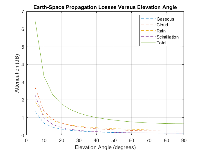
이 예제는 지구-우주 시스템을 설계할 때, 지정된 고도각 범위에 대한 지구-우주 전파 손실을 파라미터화하고 계산하는 방법을 보여줍니다.
P.618 전파 파라미터 구성하기
디폴트 P.618 구성 객체를 만듭니다. 속성값을 변경한 다음 객체 속성을 표시합니다.
cfg = p618Config;
cfg.Frequency = 14.25e9;  % Signal frequency in Hz
cfg.Latitude = 51.5;      % North direction
cfg.Longitude = -0.14;    % West direction
고도각 범위를 5도에서 90도 사이 간격으로 설정합니다.
elev_range = 5:5:90;
지구-우주 전파 손실 계산하기
지정된 구성 파라미터에 대한 지구-우주 전파 손실을 계산합니다.
elevation_angle = size(elev_range);
gaseous_attenuation = zeros(elevation_angle);
cloud_attenuation = zeros(elevation_angle);
rain_attenuation = zeros(elevation_angle);
scintillation_attenuation = zeros(elevation_angle);
total_attenuation = zeros(elevation_angle);
for  n = 1:numel(elev_range)
     cfg.ElevationAngle = elev_range(n);
     pl =  p618PropagationLosses(cfg, ...
                            'StationHeight',0.031, ...
                            'Temperature',283.6, ...
                            'Pressure',1009.48, ...
                            'WaterVaporDensity',13.79);
    gaseous_attenuation(n) = pl.Ag;
    cloud_attenuation(n) = pl.Ac;
    rain_attenuation(n) = pl.Ar;
    scintillation_attenuation(n) = pl.As;
    total_attenuation(n) = pl.At;
end
지구-우주 전파 손실 플로팅
지정된 고도각 범위에 대한 다양한 전파 손실(단위: dB)을 플로팅합니다.
plot(elev_range,gaseous_attenuation,'--');
hold on;
plot(elev_range,cloud_attenuation,'--');
hold on;
plot(elev_range,rain_attenuation,'--');
hold on;
plot(elev_range,scintillation_attenuation,'--');
hold on;
plot(elev_range,total_attenuation);
legend('Gaseous','Cloud','Rain','Scintillation','Total');
grid on;
xlabel('Elevation Angle (degrees)');
ylabel('Attenuation (dB)');
title('Earth-Space Propagation Losses Versus Elevation Angle');
초과 시간 비율에 따른 전파 손실
이 예제에서는 ITU 문서의 디지털 지도가 포함된 MAT 파일이 필요합니다. 경로에 파일이 없는 경우 다음 명령을 실행하여 MAT 파일을 다운로드하고 압축을 풉니다.
maps = exist('maps.mat','file');
p836 = exist('p836.mat','file');
p837 = exist('p837.mat','file');
p840 = exist('p840.mat','file');
matFiles = [maps p836 p837 p840];
if ~all(matFiles)
    if ~exist('ITURDigitalMaps.tar.gz','file')
        url = 'https://www.mathworks.com/supportfiles/spc/P618/ITURDigitalMaps.tar.gz';
        websave('ITURDigitalMaps.tar.gz',url);
        untar('ITURDigitalMaps.tar.gz');
    else
        untar('ITURDigitalMaps.tar.gz');
    end
    addpath(cd);
end
이 예제에서는 지구-우주 시스템을 설계할 때 시간 감쇠 값의 비율을 초과한 경우 지구-우주 전파 손실을 파라미터화하고 계산하는 방법을 보여줍니다.
지구-우주 전파 파라미터 구성하기
P.618 구성 객체를 만듭니다. 속성값을 변경한 다음 객체 속성을 표시합니다.
cfg = p618Config;
cfg.Frequency = 19.5e9;         % Signal frequency in Hz
cfg.ElevationAngle = 36.6142654;
cfg.Latitude = 46.2208;         % North direction
cfg.Longitude = 6.137;          % East direction
cfg.AntennaDiameter = 1.2;
cfg.AntennaEfficiency = 0.65;
가스 감쇠, 구름 감쇠, 강우 감쇠, 신틸레이션, 총 대기 감쇠에 대한 초과 시간 비율을 설정합니다.
annual_exceedance =[5 3 2 1 0.5 0.3 0.2 0.1 0.05 0.03 0.02 0.01 0.005 0.003 0.002 0.001];
지구-우주 전파 손실 계산하기
지정된 구성 파라미터에 대한 지구-우주 전파 손실을 계산합니다.
excess=size(annual_exceedance);
gaseous_attenuation = zeros(excess);
cloud_attenuation = zeros(excess);
rain_attenuation = zeros(excess);
scintillation=zeros(excess);
total_attenuation = zeros(excess);
for n = 1:numel(annual_exceedance)
    exceedance_value = annual_exceedance(n);
    cfg.GasAnnualExceedance = max(exceedance_value,0.1);            % Supported range is 0.1% to 99%
    cfg.CloudAnnualExceedance = max(exceedance_value,0.1);          % Supported range is 0.1% to 99%
    cfg.RainAnnualExceedance = exceedance_value;                    % Supported range is 0.001% to 5%
    cfg.ScintillationAnnualExceedance = max(exceedance_value,0.01); % Supported range is 0.01% to 5%
    cfg.TotalAnnualExceedance = exceedance_value;                   % Supported range is 0.001% to 50%
    pl =  p618PropagationLosses(cfg,'StationHeight',0.412);
    gaseous_attenuation(n) = pl.Ag;
    cloud_attenuation(n) = pl.Ac;
    rain_attenuation(n) = pl.Ar;
    scintillation(n) = pl.As;
    total_attenuation(n) = pl.At;
end
지구-우주 전파 손실 플로팅
시간 감쇠 값의 비율을 초과한 경우의 다양한 전파 손실(단위: dB)을 플로팅합니다.
loglog(annual_exceedance,gaseous_attenuation,'--');
hold on;
loglog(annual_exceedance,cloud_attenuation,'--');
hold on;
loglog(annual_exceedance,rain_attenuation,'--');
hold on;
loglog(annual_exceedance,scintillation,'--');
hold on;
loglog(annual_exceedance,total_attenuation);
legend('Gaseous','Cloud','Rain','Scintillation','Total');
grid on;
xlabel('Exceedance Probability (%)');
ylabel('Attenuation (dB)');
title('Atmospheric Losses for Time Percentage of Excess per Annum');

참고 문헌
[1] International Telecommunication Union, ITU-R Recommendation P.618 (12/2017)
[2] International Telecommunication Union, ITU-R Recommendation P.676 (08/2019)
[3] International Telecommunication Union, ITU-R Recommendation P.1511 (08/2019)
[4] International Telecommunication Union, ITU-R Recommendation P.1510 (06/2017)
[5] International Telecommunication Union, ITU-R Recommendation P.835 (12/2017)
[6] International Telecommunication Union, ITU-R Recommendation P.836 (12/2017)
[7] International Telecommunication Union, ITU-R Recommendation P.840 (08/2019)
[8] International Telecommunication Union, ITU-R Recommendation P.837 (06/2017)
[9] International Telecommunication Union, ITU-R Recommendation P.453 (08/2019)
[10] International Telecommunication Union, ITU-R Recommendation P.839 (09/2013)
[11] International Telecommunication Union, ITU-R Recommendation P.838 (03/2005)
[12] Validation examples for Study Group 3 Earth-Space propagation prediction methods, Version: 5.0 (P), ITU Radio communication Study Groups.