wcdiskmarginplot
Visualize worst-case disk-based stability margins
Syntax
Description
wcdiskmarginplot( plots the nominal and
worst-case disk-based gain and phase margins for the SISO or MIMO negative feedback loop
Lunc)feedback(Lunc,eye(N)), where N is the number of
inputs and outputs in the uncertain open-loop response Lunc.
For MIMO responses, diskmarginplot uses multiloop disk margins.
(For details about disk-based gain and phase margins, see diskmargin.)
The plot includes:
Nominal — Nominal gain and phase margins of
Lunc. The disk-based gain margin at each frequency is ±GM, where GM is the value shown in the plot in dB. Similarly, the disk-based phase margin is ±PM degrees, where PM is the value shown on the plot.Worst perturbation — The disk-based gain and phase margins for the worst perturbation within the uncertainty range
Lunc.Uncertainty. The worst perturbation corresponds to thewcuoutput argument ofwcdiskmargin. It is the perturbation that yields the smallest disk margin.Worst-case margin (lower bound) — Lower bound on the worst-case margins at each frequency. This curve represents the envelope produced by finding the smallest disk margin possible at each frequency, within the uncertainty of
Lunc.Worst-case margin (upper bound) — Upper bound on the worst-case margins at each frequency.
Sampled Uncertainty — Margins of responses randomly sampled from
Lunc.
wcdiskmarginplot(
plots the disk-based gain and phase margins computed using the skew
Lunc,sigma)sigma to bias the gain variation toward gain increase
(sigma > 0) or gain decrease (sigma < 0). If
you have used wc to obtain worst-case disk-based margins with some
particular sigma, you can use this syntax to see the frequency
dependence of the margins at that sigma value. For
sigma ≠ 0, the plotted value is GM =
min(gmax,1/max(0,gmin)). In other words, the plot shows the largest amount of
gain change [1/GM,GM] that fits within the disk-based gain margin
[gmin,gmax] of the system at the specified sigma.
wcdiskmarginplot(___, plots the
worst-case margins at the frequencies specified by w)w.
If
wis a cell array of the form{wmin,wmax}, then the plot shows the margins at frequencies ranging betweenwminandwmax.If
wis a vector of frequencies, then the plot shows the margins at each specified frequency.
wcdiskmarginplot(___, uses
specified options to customize plot elements, aspects of the worst-case margin computation,
or both. Use opts)diskmarginoptions to specify customizations for the plot.
Use wcOptions to specify customizations for the computation. You can
use this argument with any of the previous syntaxes.
Examples
Plot the worst-case disk-based gain and phase margins of the following system:
,
where a is an uncertain real parameter with a nominal value of 1 and a range of 0.2–2, and Δ is a gain-bounded dynamic uncertainty.
a = ureal('a',1,'Range',[.2 2]);
Delta = ultidyn('Delta',1);
Lunc = tf(1,[1 a 10]) * (1+0.1*Delta);

wcdiskmarginplot(Lunc)
legend('location','SouthEast')

The Worst perturbation curve corresponds to the combination of uncertain elements that yields the smallest disk margin across frequency. This perturbation corresponds to the wcu output of wcdiskmargin.
The Worst-case margin curves show the lower and upper bounds on the worst-case margins at each frequency. For any perturbation within the specified uncertainty range, the disk-based gain or phase margins of the perturbed system lie below the Worst-case margin (upper bound) curve. In other words, this curve is the envelope produced by finding the smallest margins within the uncertainty at each frequency. For this system, the lower and upper bounds are close enough to appear identical on the plot. (See wcdiskmargin for more information about these bounds.)
Focus the plot on the region between 0.5 and 10 rad/s.
w = {0.5,10};
wcdiskmarginplot(Lunc,w)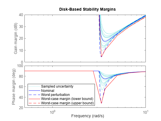
Examine the effect on the worst-case margins of increasing the uncertainty range. To do this without changing the uncertainty specified in Lunc, use the ULevel option of wcOptions. This option scales the normalized uncertainty by the factor you specify. For example, examine the worst-case margins for a 50% greater uncertainty range.
opts = wcOptions('ULevel',1.5);
wcdiskmarginplot(Lunc,w,opts)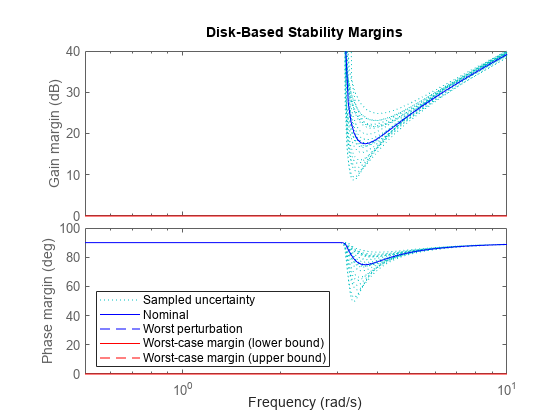
In this case, the gain and phase margins for the worst perturbation reach zero, and the worst margin at any frequency is also zero. This result means that extending the uncertainty range this far encompasses some perturbations that drive the closed-loop system feedback(Lunc,1) unstable.
Plot the worst-case disk margins as a function of frequency of a system with the following open-loop response.
a  = ureal('a',10,'PlusMinus',[-4,4]);
L = tf(25,[1 a a a]);
For the plot, use the default preferences specified in your Control System Toolbox™ preference, except specify the following attributes:
Frequency units: Hz
Gain margins on a log scale, in absolute units
Grid on
opts = diskmarginoptions('cstprefs');
opts.FreqUnits = 'Hz';
opts.MagScale = 'log';
opts.MagUnits = 'abs';
opts.grid = 'on';

w = {2*pi*1e-3,2*pi*10};   % rad/s
wcdiskmarginplot(L,w,opts)
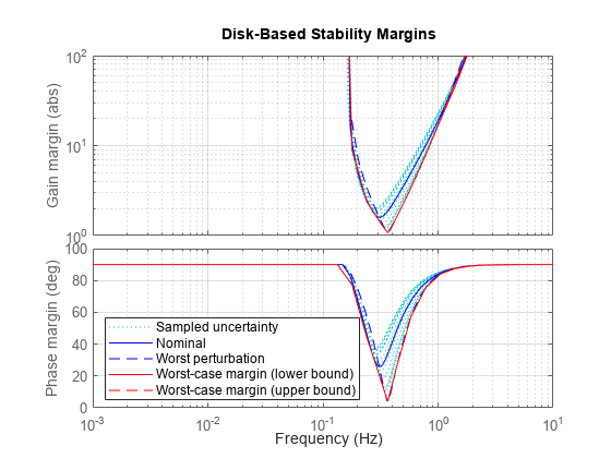
The plot you obtain might differ in appearance, depending on your current Control System Toolbox preference settings. (See Specify Toolbox Settings for Linear Analysis Plots.)
Input Arguments
Open-loop response, specified as an uncertain model such as a uss,
ufrd, genss, or genfrd
model. L can be SISO or MIMO, as long as it has the same number of
inputs and outputs. wcdiskmarginplot plots the worst-case
disk-based gain and phase margins for the negative-feedback closed-loop system
feedback(L,eye(N)).
To plot the worst-case margins of the positive feedback system
feedback(L,eye(N),+1), use
wcdiskmargin(-L).
If L is a frequency-response data model (such as
ufrd), then wcdiskmarginplot plots the
margins at each frequency represented in the model.
Skew of uncertainty region used to compute the stability margins, specified as a real scalar. This parameter biases the uncertainty used to model gain and phase variations toward gain increase or gain decrease.
The default
sigma= 0 uses a balanced model of gain variation in a range[gmin,gmax], withgmin = 1/gmax.Positive
sigmauses a model with more gain increase than decrease (gmin > 1/gmax).Negative
sigmauses a model with more gain decrease than increase (gmin < 1/gmax).
For more detailed information about how the choice of sigma
affects the margin computation, see Stability Analysis Using Disk Margins.
When plotting the gain margins of a dynamic system versus frequency, use the default
sigma = 0 to get unbiased estimates of gain and phase margins.
For sigma = 0, the worst-case disk-based gain margin at each
frequency is ±GM, where GM is the value shown in
the plot in dB.
If you have used wcdiskmargin to obtain worst-case disk-based
margins with some particular sigma, you can use this syntax to see
the frequency dependence of the margins at that sigma value. For
sigma ≠ 0, plotted value is GM =
min(gmax,1/max(0,gmin)). In other words, the plot shows the largest amount
of gain change [1/GM,GM] that fits within the disk-based gain margin
[gmin,gmax] of the system at the specified
sigma.
Frequencies at which to plot stability margins, specified as the cell array {wmin,wmax} or as a vector of frequency values.
If
wis a cell array of the form{wmin,wmax}, then the plot shows the margins at frequencies betweenwminandwmax.If
wis a vector of frequencies, then the plot shows the margins at each specified frequency. For example, uselogspaceto generate a row vector with logarithmically spaced frequency values.
Specify frequencies in units of rad/TimeUnit, where TimeUnit is the TimeUnit property of L.
Plot options, specified as:
A
diskmarginplotoptions set that you create withdiskmarginoptions. Use these options to customize aspects of plot appearance such as title, axis labels, and grids.A
wcOptionsoptions set. Use these options to customize aspects of the worst-case margins computation, such as scaling the uncertainty to examine the effect of smaller or larger uncertainty range without changing the uncertainty levels inLunc.One of each type of options set, to specify both plot options and computation options. Separate the two options sets by a comma, as in
wcdiskmarginplot(Lunc,w,plotops,compopts).
Version History
Introduced in R2020a
See Also
diskmarginplot | diskmargin | diskmarginoptions | wcdiskmargin | wcOptions