Tune and Validate Controller Parameters

The hinfstruct command lets you tune parameters in a structured control system that you have represented as a genss model with tunable elements, augmented by weighting functions that capture your design requirements. To obtain such a tunable model:

Build a genss model by creating and connecting tunable and fixed LTI models in MATLAB^®, as shown in Build Tunable Model for Tuning with hinfstruct.
Extract a genss model from a Simulink^® model using an slTuner interface, as shown in Extract Tunable Control System from Simulink Model.

Tune and Validate in Simulink

This example uses:

Open Live Script

In Simulink, use hinfstruct to tune the parameters in the genss model you extract from your Simulink model. To validate the result, write the parameters back to the model and simulate the model to evaluate the tuned performance.

To obtain the genss model, run the example Extract Tunable Control System from Simulink Model, or load the model and a preprepared slTuner interface to the model and prepared genss model of the closed-loop system with weighting functions.

open_system('rct_diskdrive')
load hinfstructTuneValidate.mat ST0 T0
T0

Generalized continuous-time state-space model with 2 outputs, 2 inputs, 13 states, and the following blocks:
  C: Tunable PID controller, 1 occurrences.
  a: Scalar parameter, 2 occurrences.

Type "ss(T0)" to see the current value and "T0.Blocks" to interact with the blocks.

Tune the tunable parameters in T0. hinfstruct finds parameter values that minimize the H-infinity norm of T0. To avoid falling into a local minimum, use the RandomStart option to restart the optimization multiple times at randomized initial parameter values.

opts = hinfstructOptions('RandomStart',5);
[T,gamma,info] = hinfstruct(T0,opts);

Final: Peak gain = 3.88, Iterations = 67
Final: Peak gain = 597, Iterations = 183
       Some closed-loop poles are marginally stable (decay rate near 1e-07)
Final: Peak gain = 597, Iterations = 173
       Some closed-loop poles are marginally stable (decay rate near 1e-07)
Final: Peak gain = 3.88, Iterations = 70
Final: Peak gain = 1.56, Iterations = 98
Final: Peak gain = 1.56, Iterations = 100

hinfstruct returns gamma equal to the smallest achieved H-infinity norm (peak gain) over all optimization runs. The function also returns the genss model T, which is a version of T0 with the tunable parameters set to the values that achieve gamma. For instance, compare the initial value of the PI controller C to the tuned value.

pid(T0.Blocks.C)

ans =
 
        1 
  Ki * ---
        s 

  with Ki = 0.001
 
Name: C
Continuous-time I-only controller.

pid(T.Blocks.C)

ans =
 
             1 
  Kp + Ki * ---
             s 

  with Kp = 0.000846, Ki = 0.0103
 
Name: C
Continuous-time PI controller in parallel form.

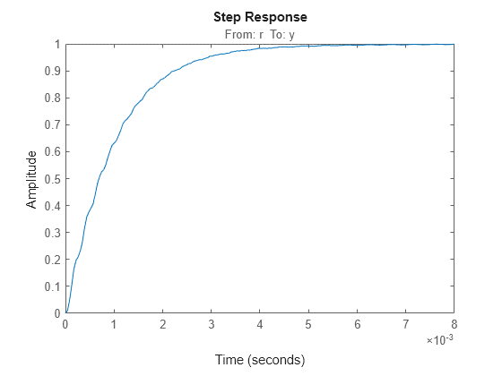
To examine the response of the linearized system with the tuned parameter values, apply the tuned values to the slTuner interface. Then extract and plot the closed-loop step response.

ST = copy(ST0);
setBlockValue(ST,T);

Try = getIOTransfer(ST,'r','y');
step(Try)

MATLAB figure

Lastly, apply the tuned values to the Simulink model to test them against the full system.

writeBlockValue(ST0)

You can now simulate the model and examine its responses with the tuned parameter values.

Tune and Validate in MATLAB

Open Live Script

In MATLAB, use hinfstruct to tune the parameters in the genss model you build by creating and connecting tunable and fixed LTI models. To validate the result, examine the responses of the open-loop or closed-loop system with the tuned parameter values.

To obtain the tunable genss model for this example, run the example Build Tunable Model for Tuning with hinfstruct, or load the prepared closed-loop model T0 and the elements of the control system, the plant G, tunable filter F, and tunable PID controller C.

load hinfstructMATLABTuneValidate T0 G F C

opts = hinfstructOptions('RandomStart',5);
[T,gamma,info] = hinfstruct(T0,opts);

Final: Peak gain = 3.88, Iterations = 67
Final: Peak gain = 597, Iterations = 190
       Some closed-loop poles are marginally stable (decay rate near 1e-07)
Final: Peak gain = 597, Iterations = 186
       Some closed-loop poles are marginally stable (decay rate near 1e-07)
Final: Peak gain = 1.56, Iterations = 123
Final: Peak gain = 1.56, Iterations = 98
Final: Peak gain = 1.56, Iterations = 98

pid(T0.Blocks.C)

ans =
 
        1 
  Ki * ---
        s 

  with Ki = 0.001
 
Name: C
Continuous-time I-only controller.

pid(T.Blocks.C)

ans =
 
             1 
  Kp + Ki * ---
             s 

  with Kp = 0.000846, Ki = 0.0103
 
Name: C
Continuous-time PI controller in parallel form.

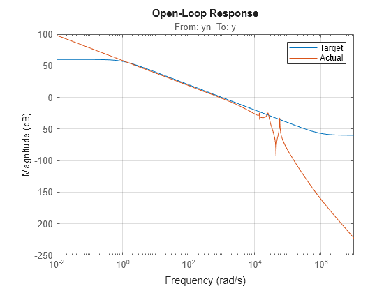
To validate the result, compare the unweighted open-loop response with the target open-loop response, which for T0 was specified as:

$LS = \frac{1 + 0.001 \frac{s}{ω_{c}}}{0.001 + \frac{s}{ω_{c}}}$

(See Build Tunable Model for Tuning with hinfstruct.)

wc = 1000; 
s = tf('s');
LS = (1+0.001*s/wc)/(0.001+s/wc);

Construct the open-loop response with the tuned parameter values. Because C is itself a tuned block, you can get its tuned value directly from T. F is a genss model with tunable parameter a, so you must use getValue to propagate the value of the tunable parameter in T to F.

C = getBlockValue(T,'C');
F = getValue(F,T.Blocks); 

L = G*C*F;

bodemag(LS,L) 
grid on
title('Open-Loop Response') 
legend('Target','Actual')

MATLAB figure

The 0dB crossover frequency and overall loop shape are as expected. Finally, plot the step response of the overall closed-loop system using the tuned parameter values.

CL = feedback(G*C,F);
step(CL)
grid on
title('Closed-Loop Response')

MATLAB figure