MIMO Robustness Analysis
You can create and analyze uncertain state-space models made up of uncertain state-space matrices. In this example, create a MIMO system with parametric uncertainty and analyze it for robust stability and worst-case performance.
Consider a two-input, two-output, two-state system whose model has parametric uncertainty in the state-space matrices. First create an uncertain parameter p. Using the parameter, make uncertain A and C matrices. The B matrix happens to be not-uncertain, although you will add frequency-domain input uncertainty to the model later.
p = ureal('p',10,'Percentage',10);
A = [0 p;-p 0];
B = eye(2);
C = [1 p;-p 1];
H = ss(A,B,C,[0 0;0 0])
Uncertain continuous-time state-space model with 2 outputs, 2 inputs, 2 states.
The model uncertainty consists of the following blocks:
  p: Uncertain real, nominal = 10, variability = [-10,10]%, 2 occurrences
Model Properties

Type "H.NominalValue" to see the nominal value and "H.Uncertainty" to interact with the uncertain elements.
You can view the properties of the uncertain system H using the get command.
get(H)
     NominalValue: [2×2 ss]
      Uncertainty: [1×1 struct]
                A: [2×2 umat]
                B: [2×2 double]
                C: [2×2 umat]
                D: [2×2 double]
                E: []
        StateName: {2×1 cell}
        StateUnit: {2×1 cell}
    InternalDelay: [0×1 double]
       InputDelay: [2×1 double]
      OutputDelay: [2×1 double]
        InputName: {2×1 cell}
        InputUnit: {2×1 cell}
       InputGroup: [1×1 struct]
       OutputName: {2×1 cell}
       OutputUnit: {2×1 cell}
      OutputGroup: [1×1 struct]
            Notes: [0×1 string]
         UserData: []
             Name: ''
               Ts: 0
         TimeUnit: 'seconds'
     SamplingGrid: [1×1 struct]
Most properties behave in the same way as the corresponding properties of ss objects. The property NominalValue is itself an ss object.
Adding Independent Input Uncertainty to Each Channel
The model for H does not include actuator dynamics. Said differently, the actuator models are unity-gain for all frequencies.
Nevertheless, the behavior of the actuator for channel 1 is modestly uncertain (say 10%) at low frequencies, and the high-frequency behavior beyond 20 rad/s is not accurately modeled. Similar statements hold for the actuator in channel 2, with larger modest uncertainty at low frequency (say 20%) but accuracy out to 45 rad/s.
Use ultidyn objects Delta1 and Delta2 along with shaping filters W1 and W2 to add this form of frequency domain uncertainty to the model.
W1 = makeweight(.1,20,50);
W2 = makeweight(.2,45,50);
Delta1 = ultidyn('Delta1',[1 1]);
Delta2 = ultidyn('Delta2',[1 1]);
G = H*blkdiag(1+W1*Delta1,1+W2*Delta2)
Uncertain continuous-time state-space model with 2 outputs, 2 inputs, 4 states.
The model uncertainty consists of the following blocks:
  Delta1: Uncertain 1x1 LTI, peak gain = 1, 1 occurrences
  Delta2: Uncertain 1x1 LTI, peak gain = 1, 1 occurrences
  p: Uncertain real, nominal = 10, variability = [-10,10]%, 2 occurrences
Model Properties

Type "G.NominalValue" to see the nominal value and "G.Uncertainty" to interact with the uncertain elements.
Note that G is a two-input, two-output uncertain system, with dependence on three uncertain elements, Delta1, Delta2, and p. It has four states, two from H and one each from the shaping filters W1 and W2, which are embedded in G.
You can plot a 2-second step response of several samples of G The 10% uncertainty in the natural frequency is apparent.
stepplot(G,2)

You can create a Bode plot of samples of G. The high-frequency uncertainty in the model is also apparent. For clarity, start the Bode plot beyond the resonance.
bodeplot(G,{13 100})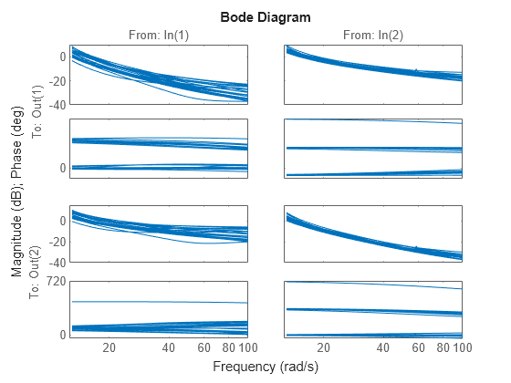
Closed-Loop Robustness Analysis
Load the controller and verify that it is two-input and two-output.
load('mimoKexample.mat')
size(K)
State-space model with 2 outputs, 2 inputs, and 9 states.
You can use the command loopsens to form all the standard plant/controller feedback configurations, including sensitivity and complementary sensitivity at both the input and output. Because G is uncertain, all the closed-loop systems are uncertain as well.
F = loopsens(G,K)
F = struct with fields:
        Si: [2×2 uss]
        Ti: [2×2 uss]
        Li: [2×2 uss]
        So: [2×2 uss]
        To: [2×2 uss]
        Lo: [2×2 uss]
       PSi: [2×2 uss]
       CSo: [2×2 uss]
     Poles: [13×1 double]
    Stable: 1
F is a structure with many fields. The poles of the nominal closed-loop system are in F.Poles, and F.Stable is 1 if the nominal closed-loop system is stable. In the remaining 10 fields, S stands for sensitivity, T or complementary sensitivity, and L for open-loop gain. The suffixes i and o refer to the input and output of the plant. Finally, P and C refer to the plant and controller.
Hence, Ti is mathematically the same as:
.
Lo is G*K, and CSo is mathematically the same as
.
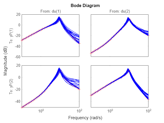
Examine the transmission of disturbances at the plant input to the plant output by plotting responses of F.PSi. Graph some samples along with the nominal.
bodemag(F.PSi.NominalValue,'r+',F.PSi,'b-',{1e-1 100})
Nominal Stability Margins
You can use allmargin to investigate loop-at-a-time gain and phase margins, and diskmargin for loop-at-a-time disk-based margins and simultaneous multivariable margins. Margins are computed for the nominal system and do not reflect the uncertainty models within G.
For instance, explore the disk-based margins for gain or phase variations at the plant outputs and inputs. (For general information about disk-based margin analysis, see Stability Analysis Using Disk Margins.)
[DMo,MMo] = diskmargin(G*K);
[DMi,MMi] = diskmargin(K*G);
The loop-at-a-time margins are returned in the structure arrays DMo and DMi. Each of these arrays contains one entry for each of the two feedback channels. For instance, examine the margins at the plant output for the second feedback channel.
DMo(2)
ans = struct with fields:
           GainMargin: [0.0682 14.6726]
          PhaseMargin: [-82.2022 82.2022]
           DiskMargin: 1.7448
           LowerBound: 1.7448
           UpperBound: 1.7448
            Frequency: 4.8400
    WorstPerturbation: [2×2 ss]
This result tells you that the gain at the second plant output can vary by factors between about 0.07 and about 14.7, without the second loop going unstable. Similarly, the loop can tolerate phase variations at the output up to about ±82°.
The structures MMo and MMi contain the margins for concurrent and independent variations in both channels. For instance, examine the multiloop margins at the plant inputs.
MMi
MMi = struct with fields:
           GainMargin: [0.1186 8.4289]
          PhaseMargin: [-76.4682 76.4682]
           DiskMargin: 1.5758
           LowerBound: 1.5758
           UpperBound: 1.5790
            Frequency: 5.9828
    WorstPerturbation: [2×2 ss]
This result tells you that the gain at the plant input can vary in both channels independently by factors between about 1/8 and 8 without the closed-loop system going unstable. The system can tolerate independent and concurrent phase variations up about ±76°. Because the multiloop margins take loop interactions into account, they tend to be smaller than loop-at-a-time margins.
Examine the multiloop margins at the plant outputs.
MMo
MMo = struct with fields:
           GainMargin: [0.1201 8.3290]
          PhaseMargin: [-76.3074 76.3074]
           DiskMargin: 1.5712
           LowerBound: 1.5712
           UpperBound: 1.5744
            Frequency: 17.3984
    WorstPerturbation: [2×2 ss]
The margins at the plant outputs are similar to those at the inputs. This result is not always true in multiloop feedback systems.
Finally, examine the margins against simultaneous variations at the plant inputs and outputs.
MMio = diskmargin(G,K)
MMio = struct with fields:
           GainMargin: [0.5676 1.7619]
          PhaseMargin: [-30.8440 30.8440]
           DiskMargin: 0.5517
           LowerBound: 0.5517
           UpperBound: 0.5528
            Frequency: 9.0688
    WorstPerturbation: [1×1 struct]
When you consider all such variations simultaneously, the margins are somewhat smaller than those at the inputs or outputs alone. Nevertheless, these numbers indicate a generally robust closed-loop system. The system can tolerate significant simultaneous gain variations or ±30° degree simultaneous phase variations in all input and output channels of the plant.
Robust Stability Margin
With diskmargin, you determine various stability margins of the nominal multiloop system. These margins are computed only for the nominal system and do not reflect the uncertainty explicitly modeled by the ureal and ultidyn objects. When you work with a detailed uncertainty model, the stability margins computed by diskmargin may not accurately reflect how close the system is from being unstable. You can then use robstab to compute the robust stability margin for the specified uncertainty.
In this example, use robstab to compute the robust stability margin for the uncertain feedback loop comprised of G and K. You can use any of the closed-loop transfer functions in F = loopsens(G,K). All of them, F.Si, F.To, etc., have the same internal dynamics, and hence their stability properties are the same.
opt = robOptions('Display','on');
stabmarg = robstab(F.So,opt)
Computing peak...  Percent completed: 100/100
System is robustly stable for the modeled uncertainty.
 -- It can tolerate up to 221% of the modeled uncertainty.
 -- There is a destabilizing perturbation amounting to 222% of the modeled uncertainty.
 -- This perturbation causes an instability at the frequency 13.6 rad/seconds.
stabmarg = struct with fields:
           LowerBound: 2.2129
           UpperBound: 2.2173
    CriticalFrequency: 13.6336
This analysis confirms what the diskmargin analysis suggested. The closed-loop system is quite robust, in terms of stability, to the variations modeled by the uncertain parameters Delta1, Delta2, and p. In fact, the system can tolerate more than twice the modeled uncertainty without losing closed-loop stability.
Worst-Case Gain Analysis
You can plot the Bode magnitude of the nominal output sensitivity function. It clearly shows decent disturbance rejection in all channels at low frequency.
bodemag(F.So.NominalValue,{1e-1 100})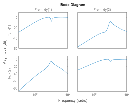
You can compute the peak value of the maximum singular value of the frequency response matrix using norm.
[PeakNom,freq] = getPeakGain(F.So.NominalValue)
PeakNom =
1.1317
freq =
7.1300
The peak is about 1.13. What is the maximum output sensitivity gain that is achieved when the uncertain elements Delta1, Delta2, and p vary over their ranges? You can use wcgain to answer this.
[maxgain,wcu] = wcgain(F.So);
maxgain
maxgain = struct with fields:
           LowerBound: 2.1599
           UpperBound: 2.1643
    CriticalFrequency: 8.3357
The analysis indicates that the worst-case gain is somewhere between 2.1 and 2.2. The frequency where the peak is achieved is about 8.5.
Use usubs to replace the values for Delta1, Delta2, and p that achieve the gain of 2.1. Make the substitution in the output complementary sensitivity, and do a step response.
step(F.To.NominalValue,usubs(F.To,wcu),5)
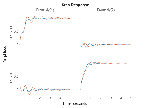
The perturbed response, which is the worst combination of uncertain values in terms of output sensitivity amplification, does not show significant degradation of the command response. The settling time is increased by about 50%, from 2 to 4, and the off-diagonal coupling is increased by about a factor of about 2, but is still quite small.
You can also examine the worst-case frequency response alongside the nominal and sampled systems using wcsigmaplot.
wcsigmaplot(F.To,{1e-1,100})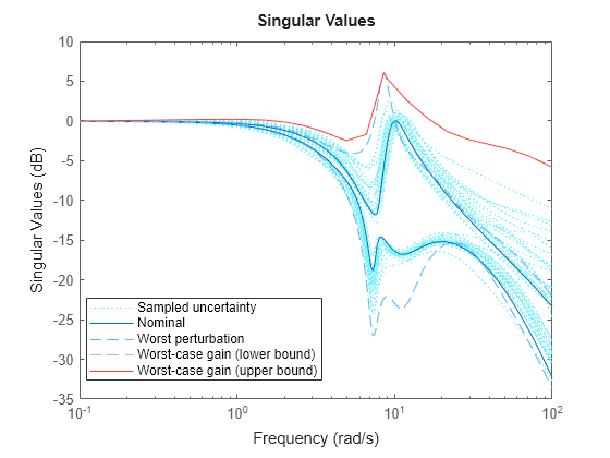
See Also
ultidyn | loopsens | diskmargin | robstab | wcgain | usubs | wcsigmaplot