Perform Profit-and-Loss Attribution Test
This example shows how to apply the Fundamental Review of the Trading Book (FRTB) profit-and-loss (P&L) attribution test to the recent trading history of a portfolio. The P&L attribution test determines whether two empirical distributions containing different P&L measures are similar enough for the measures to be considered equivalent for regulatory purposes. One distribution contains risk theoretical P&L (RTPL) values, which are the portfolio losses calculated by the trading desk's internal valuation model at the end of the trading period. The other distribution contains hypothetical P&L (HPL) values, which are the losses the portfolio would realize if the portfolio did not buy or sell any assets over the trading period. Profits are represented by negative P&L values.
Load P&L Data
Load the profit-and-loss data.
load("PandLValues.mat");The vectors HPL and RTPL contain HPL and RTPL data for 250 trading days, or one year, of a simulated portfolio.
Plot the HPL data against RTPL data with a line representing equality between the axes.
x = linspace(-4E4,3E4,100);

plot(RTPL,HPL,"o");
hold on
plot(x,x)
xlabel("RTPL");
ylabel("HPL");
title("HPL vs. RTPL");
hold off
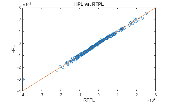
The data in HPL and RTPL are clustered around the equality, which suggests that they might be equivalent measures in a regulatory context.
Calculate Spearman Rank Correlation
The P&L attribution test uses the Spearman rank correlation between the observations in HPL and RTPL. The Spearman rank correlation is equivalent to calculating Pearson's linear correlation for the HPL and RTPL rankings.
Plot the HPL ranks against the RTPL ranks and calculate the Spearman rank correlation using the risk.validation.plotSpearmanRanks function.
risk.validation.plotSpearmanRanks(RTPL,HPL);
title("P&L Attribution Test: Spearman Correlation");
xlabel("RTPL Rank")
ylabel("HPL Rank")
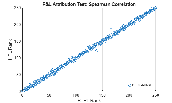
The ranks appear to have a positive linear relationship, which is consistent with the very high Spearman rank correlation of 0.99879.
Use the Statistics and Machine Learning Toolbox™ corr function to save the Spearman rank correlation in the workspace variable r.
r = corr(HPL,RTPL,"Type","Spearman");
Calculate Kolmogorov Smirnov Metric
The P&L attribution test also uses the Kolmogorov-Smirnov (KS) metric. The KS metric is the largest absolute difference between two empirical CDFs, evaluated at the same value of the distributions' random variable. In a P&L context, the KS metric is the distance between the CDFs for the HPL and RTPL data. For more information, see the Algorithms section in risk.validation.kolmogorovSmirnov.
Plot the empirical CDFs for HPL and RTPL together with a profile of their absolute differences by using the risk.validation.kolmogorovSmirnovPlot function. Specify a difference threshold of 0.09, which is the upper bound of the FRTB green zone for the KS metric. The green zone corresponds to values for the KS metric, which indicates the HPL and RTPL measures are equivalent for regulatory purposes.
risk.validation.kolmogorovSmirnovPlot(HPL,RTPL,"PlotDifferences",true,"DifferenceThresholds",0.09);
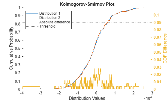
The left axes contain the empirical CDFs for the HPL and RTPL data, which correspond to the legend entries Distribution 1 and Distribution 2, respectively. The absolute differences between the empirical CDFs are plotted in the right axes together with the difference threshold, which the plot represents as a dashed line. The KS metric, which is the maximum of the absolute differences, is between 0.02 and 0.04 and below the threshold.
Calculate the KS metric for the data in HPL and RTPL using the risk.validation.kolmogorovSmirnov function.
KSValue = risk.validation.kolmogorovSmirnov(HPL,RTPL)
KSValue =
0.0280
The value for the KS metric is 0.0280, which is consistent with the results in the plot.
Perform P&L attribution test
The P&L attribution test uses the following three zones to classify the Spearman correlation and KS metrics:
The green zone corresponds to a Spearman correlation greater than
0.8and a KS metric less than0.09. Metrics that fall into the green zone do not indicate the presence of quality or accuracy issues with the bank's risk model.The red zone corresponds to a Spearman correlation of less than
0.7or a KS metric of greater than0.12. Metrics that fall into the red zone definitively indicate the presence of issues with the bank's risk model.The amber zone corresponds to Spearman correlation and KS metric pairs that do not fall into the green or red zones. Metrics that fall into the amber zone indicate the possibility of issues with the bank's risk model.
Use the PLATestZone helper function to classify r and KSValue.
zoneColor = PLATestZone(r,KSValue)
zoneColor =
"green"
The output indicates that the HPL and RTPL measures are equivalent for regulatory purposes.
Helper Functions
This code defines the PLATestZone function, which classifies the Spearman correlation and KS metric for a FRTB P&L attribution test.
function zoneColor = PLATestZone(r,KSvalue)

    if KSvalue < .09 && r > 0.8
        zoneColor = "green";
    elseif r < 0.7 || KSvalue > 0.12
        zoneColor = "red";
    else
        zoneColor = "amber";
    end

end
See Also
risk.validation.plotSpearmanRanks | risk.validation.kolmogorovSmirnovPlot | risk.validation.kolmogorovSmirnov | detectdrift | corr