Analyze Nolen Matrix for the 2-D Beamforming Application
The Nolen matrix is a novel antenna feeding network composed of only couplers with dedicated coupling ratios and phase shifters. In this example a 2D beamforming array using planar Nolen matrix [1] designed at 2 GHz, is imported and analyzed. The proposed 3 ×3 Nolen matrix is saved in the gerber file and analyzed at 2 GHz with FR4 substrate. All simulation results are matched with the design theory[1] and the measured result.
Import the gerber file and create Nolen Matrix.
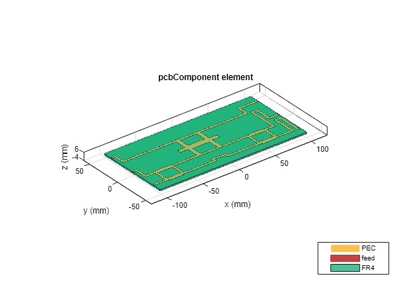
The imported 3x3 Nolen matrix planar array with three input ports and three output ports consists of three hybrid couplers and three phase shifters in a layouti, in order to achieve the equal magnitude and progressive phase shifts at output ports. For couplers, one with coupling ratio 2/3 is placed at the top of the layout, while the other two with coupling ratio 1/2 are at the bottom.Three transmission lines with 50-ohm characteristic impedance and electrical length of 90, 90 for symmetry and 125.83deg are used as phase delay lines that connect the adjacent couplers.
Import the gerber file using gerberRead, and convert it to pcbComponent
P = gerberRead("NolenMatrixShape.gtl","NolenMatrixShape.gbl");
S = P.StackUp;
S.Layer3  = dielectric("Name",'FR4',"EpsilonR",4.8,"LossTangent",0.0026,"Thickness",0.0016);
P.StackUp = S;

% Create pcbComponent
Nolen = pcbComponent(P);
L = Nolen.Layers;
substrate = L{3};
% Set Board thickness
Nolen.BoardThickness = substrate.Thickness;
Nolen.Layers = {L{2},L{3},L{4}};

feedloc = [[-0.101 0.03717095 1 3];...
    [-0.101 -0.0002651007 1 3];...
    [-0.101 -0.03752398 1 3];...
    [0.101 0.0371732 1 3];...
    [0.101 4.674166e-05 1 3];...
    [0.101 -0.03748122 1 3]];
Nolen.FeedLocations = feedloc;
Nolen.FeedDiameter = 0.00295/2;
Display PCB structure
figure;show(Nolen)
Comparison of simulated result with Measured result
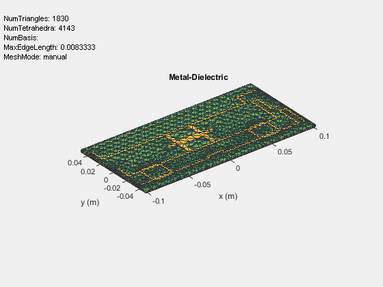
Mesh the structure using manual meshing with MaxEdgeLength of lambda/18.
plotfrequency = 2*1e9;
lambda = 3e8/plotfrequency;
% Manual mesh
figure; mesh(Nolen,'MaxEdgeLength',lambda/18);
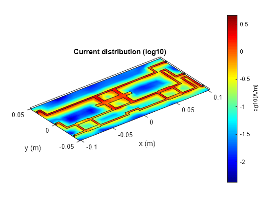
Compute current at design frequency 2Ghz
% Current at 2Ghz
figure; current(Nolen,2e9,scale="log10")
Measurement - Sparameters and Phase
The designed Nolen matrix planar array is fabricated using FR4 susbtrate. The scattering parameters of fabricated structure is measured using a Network Analyzer. The figure below shows the top view of the fabricated Nolen matrix

Measured sparameters at 2GHz
Load the .mat file with measured data.
SMeasured = load('SparamsMeasured.mat');
SparamsM = SMeasured.SparamsMeasured;
Compute simulated sparameters at 2GHz
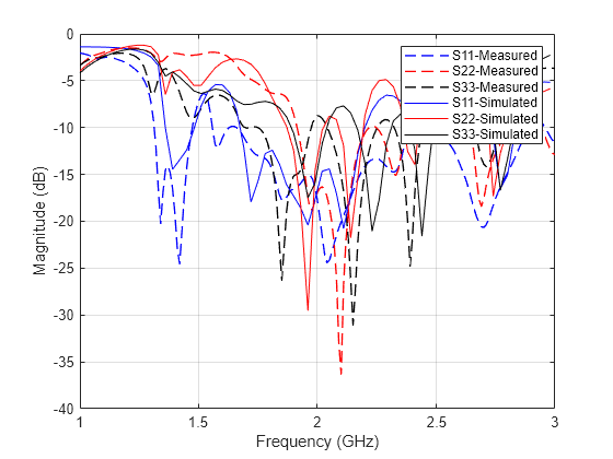
The sparameters are analyzed with the frequency sweep of 1-3 Ghz, the insertion loss at output ports w.r.t the input port1, 2 and 3 is analyzed.
frequencyRange = (1:0.03:3)*1e9;
sparSimu = sparameters(Nolen,frequencyRange);
Plot the measured and simulated return loss for input port1, port2 and port3
% Measured Return loss w.r.t input ports
Freq = SparamsM.Freq;
S11_meas = SparamsM.S11_meas;
S22_meas = SparamsM.S22_meas;
S33_meas = SparamsM.S33_meas;
figure; plot(Freq,S11_meas,'b--',"LineWidth",1);
hold on; plot(Freq,S22_meas,'r--',"LineWidth",1);
hold on; plot(Freq,S33_meas,'k--',"LineWidth",1);
% Simulated Return loss w.r.t input ports
hold on; rfplot(sparSimu,1,1,'b');
hold on; rfplot(sparSimu,2,2,'r');
hold on; rfplot(sparSimu,3,3,'k');
legend('S11-Measured','S22-Measured','S33-Measured','S11-Simulated','S22-Simulated','S33-Simulated');
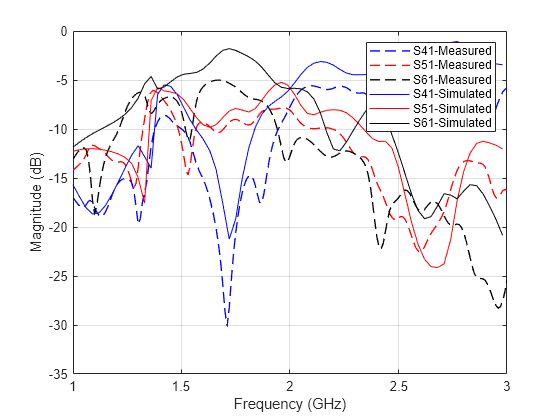
Plot the measured and simulated insertion loss at output ports 4, 5 and 6 w.r.t input port1
% Measured Insertion loss at port4, port5 and port6 w.r.t port1
S41_meas = SparamsM.S41_meas;
figure; plot(Freq,S41_meas,'b--',"LineWidth",1);
S51_meas = SparamsM.S51_meas;
hold on; plot(Freq,S51_meas,'r--',"LineWidth",1);
S61_meas = SparamsM.S61_meas;
hold on; plot(Freq,S61_meas,'k--',"LineWidth",1);
grid on;
% Simulated Insertion loss at port4, port5 and port6 w.r.t port1
hold on; rfplot(sparSimu,4,1,'b');
hold on; rfplot(sparSimu,5,1,'r');
hold on; rfplot(sparSimu,6,1,'k');
legend('S41-Measured','S51-Measured','S61-Measured','S41-Simulated','S51-Simulated','S61-Simulated');
Plot the measured and simulated insertion loss at output ports 4, 5 and 6 w.r.t input port2
% Measured Insertion loss at port4, port5 and port6 w.r.t port2
S42_meas = SparamsM.S24_meas;
figure; plot(Freq,S42_meas,'b--',"LineWidth",1);
S52_meas = SparamsM.S25_meas;
hold on; plot(Freq,S52_meas,'r--',"LineWidth",1);
S62_meas = SparamsM.S26_meas;
hold on; plot(Freq,S62_meas,'k--',"LineWidth",1);
grid on;hold on;
% Simulated Insertion loss at port4, port5 and port6 w.r.t port2
rfplot(sparSimu,2,4,'b');hold on;
rfplot(sparSimu,2,5,'r');hold on;
rfplot(sparSimu,2,6,'k');hold on;
legend('S42-Measured','S52-Measured','S62-Measured','S42-Simulated','S52-Simulated','S62-Simulated');

Plot the measured and simulated insertion loss at output ports 4, 5 and 6 w.r.t input port3
% Measured Output at port4, port5 and port6 w.r.t port3
S43_meas = SparamsM.S34_meas;
figure; plot(Freq,S43_meas,'b--',"LineWidth",1);
S53_meas = SparamsM.S35_meas;
hold on; plot(Freq,S53_meas,'r--',"LineWidth",1);
S63_meas = SparamsM.S36_meas;
hold on; plot(Freq,S63_meas,'k--',"LineWidth",1);
grid on;hold on;
% Simulated Insertion loss at port4, port5 and port6 w.r.t port3
rfplot(sparSimu,3,4,'b');hold on;
rfplot(sparSimu,3,5,'r');hold on;
rfplot(sparSimu,3,6,'k');hold on; legend('S34-Measured','S35-Measured','S36-Measured','S34-Simulated','S35-Simulated','S36-Simulated')
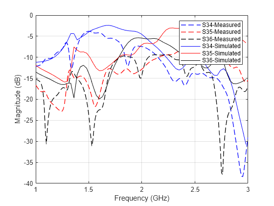
The designed Nolen Matrix is simulated in the frequency span of 1-3GHz. It is observed that the return loss for three ports are below 14dB while the insertion loss at the outputs is between 6-8dB respectively.
Compute phase at 2GHz
The simulated phase difference that are obtained between output ports due to input ports.
% w.r.t Port1
figure; plot(sparSimu.Frequencies,(((angle(rfparam(sparSimu,5,1)))-(angle(rfparam(sparSimu,4,1))))*180/pi));
hold on;
plot(sparSimu.Frequencies,(((angle(rfparam(sparSimu,6,1)))-(angle(rfparam(sparSimu,5,1))))*180/pi));
legend('(phase51-phase41)simu','(phase61-phase51)simu')
grid on;

% w.r.t Port2
figure; plot(sparSimu.Frequencies,(((angle(rfparam(sparSimu,5,2)))-(angle(rfparam(sparSimu,4,2))))*180/pi));
hold on;grid on;
plot(sparSimu.Frequencies,(((angle(rfparam(sparSimu,6,2)))-(angle(rfparam(sparSimu,5,2))))*180/pi));
legend('(phase52-phase42)simu','(phase62-phase52)simu')

% w.r.t Port3
figure; plot(sparSimu.Frequencies,(((angle(rfparam(sparSimu,5,3)))-(angle(rfparam(sparSimu,4,3))))*180/pi));
hold on;grid on;
plot(sparSimu.Frequencies,(((angle(rfparam(sparSimu,6,3)))-(angle(rfparam(sparSimu,5,3))))*180/pi));
legend('(phase53-phase43)simu','(phase63-phase53)simu')
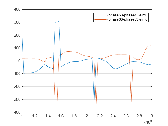
The below table shows the phase differences between the adjacent output ports, when the input ports P1, P2, and P3 are excited.
Ports Excited | Phase(51)-Phase(41) (deg) | Phase(61)-Phase(51) (deg) |
Port1 | 86.86 | 86.86 |
Port2 | 135.23 | -206.12 (153.88) |
Port3 | 15.93 | 33.70 |
% measured Phase difference between adjacent ports
% Needs to add this
Conclusion
A 3×3 Nolen matrix is simulated and compared with the measured results. It is observed that the simulated results matched well with the measured results. The structure exhibits relatively equal magnitude and three different phase differences between adjacent outputs by exciting three input ports which makes it a suitable candidate for 2D beamforming application.
You can also select a web site from the following list
Americas
- América Latina (Español)
- Canada (English)
- United States (English)
Europe
- Belgium (English)
- Denmark (English)
- Deutschland (Deutsch)
- España (Español)
- Finland (English)
- France (Français)
- Ireland (English)
- Italia (Italiano)
- Luxembourg (English)
- Netherlands (English)
- Norway (English)
- Österreich (Deutsch)
- Portugal (English)
- Sweden (English)
- Switzerland
- United Kingdom (English)
Asia Pacific
- Australia (English)
- India (English)
- New Zealand (English)
- 中国
- 日本Japanese (日本語)
- 한국Korean (한국어)