Bisect S-Parameters of Cascaded Probes
This example shows how to separate the S-parameters of two identical, passive, symmetric probes connected in a cascade.
Introduction
Consider a DUT (device under test) connected to two probes. In order to de-embed the S-parameters of DUT, you need to know the S-parameters of each individual probe. For accurate S-parameters of the two probes, the calibration is done in the lab using SOLT (short, open, load, and thru) or TRL (thru, reflect, line) measurements. However, if you assume the probes are identical and symmetric, then you can approximate S-parameters quickly using the procedure sketched here.
The file connectedprobes.s2p contains the S-parameter data when the probes are connected directly to each other.
ABCD-parameters
This example uses ABCD-parameters to bisect measured S-parameter data into the data for each individual probe.
When you cascade two networks, you can calculate the ABCD-parameters of the combined network by matrix multiplying the ABCD-parameters of the two individual networks.

Figure 1: Main network and network with two symmetric probes connected in a cascade
If, , then,
From the above equation, you can find the ABCD-parameters of the two individual probes by taking the matrix square root of the ABCD-parameters of main network.
Since both probes are identical, you can calculate the S-parameters of either one of the probes.
Extract Required S-Parameter Data from Given Touchstone file
Create an sparameters object from the Touchstone® data file connectedprobes.s2p.
filename = 'connectedprobes.s2p';
S = sparameters(filename);
numports = S.NumPorts;
freq = S.Frequencies;
numfreq = numel(freq);
z0 = S.Impedance;
Calculate S-Parameter Data of Individual Probe
Create a zero matrix to store the ABCD-parameter data of the probe.
abcd_probe_data = zeros(numports,numports,numfreq);
To calculate S-Parameters of the probe, you need to know the S-parameters at every frequency it operates. Convert the S-parameters extracted from connectedprobes.s2p to ABCD-parameters. Then calculate the matrix square root of ABCD-parameters using sqrtm function to get the ABCD-parameters of the probe. Convert these ABCD-parameters of the probe to S-parameters.
ABCD = abcdparameters(S);
for n = 1:numfreq
    abcd_meas = ABCD.Parameters(:,:,n);
    abcd_probe_data(:,:,n) = sqrtm(abcd_meas);
end
ABCD_probe = abcdparameters(abcd_probe_data,freq);
Create an S-parameter object from the calculated S-parameter data of the probe.
S_probe = sparameters(ABCD_probe,z0);
Compare Calculated S-Parameters with Expected S-Parameters
For this example, connectedprobes.s2p gives the S-Parameter data of this network.

Figure 2: Network derived from connectedprobes.s2p
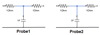
Split the above network into two identical networks, probe1 and probe2. The S-parameters of these probes represent the expected result.

Figure 3: Identical Networks
Create probe1 using circuit, resistor, and capacitor objects from the RF Toolbox.
R1 = 1;
C1 = 1;
R2 = 1;
ckt = circuit('probe1');
add(ckt,[1 2],resistor(R1))
add(ckt,[2 4],capacitor(C1))
add(ckt,[2 3],resistor(R2))
Calculate the expected S-parameters of probe 1.
setports(ckt,[1 4],[3 4])
S_exp = sparameters(ckt,freq,z0);
Plot and compare the expected S-parameters from probe1 and those calculated using ABCD-parameters and compare.
rfplot(S_exp,'+')
hold on
rfplot(S_probe,'--')
hold off
text(40,-30,{'+: Expected','--: Computed'})

Compare Cascaded S-Parameters of Probe1 with S-Parameters of Combined Network
Cascade S-parameters of probe1 with itself using cascadesparams function and create an S-parameter object with cascaded S-parameters.
S_combined = cascadesparams(S_probe,S_probe);
Plot and compare S-parameters from connectedprobes.s2p and those calculated from combined probe1.
figure
rfplot(S,'+')
hold on
rfplot(S_combined,'--')
hold off
text(40,-27,{'+: Expected','--: Computed'})

Limitations
The procedure shown here cannot replace traditional calibration. We include it as an example of using RF Toolbox™ and MATLAB™ to manipulate network parameters mathematically.
There are some limitations to using this procedure.
There is no guaranteed solution. Some matrices do not have a square root.
The solution may not be unique. Often, there are two or more viable matrix square roots.