이 번역 페이지는 최신 내용을 담고 있지 않습니다. 최신 내용을 영문으로 보려면 여기를 클릭하십시오.
accelerate
설명
newAppx = accelerate(oldAppx,useAcceleration)oldAppx와 동일한 구성을 갖는 새로운 신경만 기반 함수 근사기 객체 newAppx를 반환하고 기울기 계산 속도를 높이는 옵션(논리값 useAcceleration)을 설정합니다.
예제
Q-값 함수에 대한 기울기 계산 속도 높이기
관측값 및 행동 사양 객체를 만듭니다. (또는 getObservationInfo 및 getActionInfo를 사용하여 환경에서 사양 객체를 추출합니다.) 이 예제에서는 2개 채널을 갖는 관측값 공간을 정의합니다. 첫 번째 채널은 4차원 연속 공간의 관측값을 전달합니다. 두 번째 채널은 0 또는 1일 수 있는 이산 스칼라 관측값을 전달합니다. 마지막으로, 행동 공간은 연속 행동 공간의 3차원 벡터입니다.
obsInfo = [rlNumericSpec([4 1])
           rlFiniteSetSpec([0 1])];

actInfo =  rlNumericSpec([3 1]);
크리틱 내에서 Q-값 함수를 근사하기 위해 순환 심층 신경망을 만듭니다. 출력 계층은 주어진 관측값에 대해 실행할 행동의 가치를 표현하는 스칼라여야 합니다.
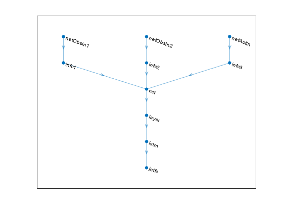
각 신경망 경로를 layer 객체로 구성된 배열로 정의합니다. 환경 사양 객체에서 관측값 공간과 행동 공간의 차원을 가져오고, 나중에 적절한 환경 채널과 명시적으로 연결할 수 있도록 입력 계층의 이름을 지정합니다. 신경망이 순환 신경망이므로, sequenceInputLayer를 입력 계층으로 사용하고 lstmLayer를 다른 신경망 계층 중 하나로 포함합니다.
% Define paths
inPath1 = [ sequenceInputLayer( ...
                prod(obsInfo(1).Dimension), ...
                Name="netObsIn1")
            fullyConnectedLayer(5,Name="infc1") ];

inPath2 = [ sequenceInputLayer( ...
                prod(obsInfo(2).Dimension), ...
                Name="netObsIn2")
            fullyConnectedLayer(5,Name="infc2") ];

inPath3 = [ sequenceInputLayer( ...
                prod(actInfo(1).Dimension), ...
                Name="netActIn")
            fullyConnectedLayer(5,Name="infc3") ];

% Concatenate 3 previous layer outputs along dim 1
jointPath = [ concatenationLayer(1,3,Name="cct")
              tanhLayer
              lstmLayer(8,"OutputMode","sequence")
              fullyConnectedLayer(1,Name="jntfc") ];

% Add layers to network object
net = layerGraph;
net = addLayers(net,inPath1);
net = addLayers(net,inPath2);
net = addLayers(net,inPath3);
net = addLayers(net,jointPath);

% Connect layers
net = connectLayers(net,"infc1","cct/in1");
net = connectLayers(net,"infc2","cct/in2");
net = connectLayers(net,"infc3","cct/in3");

% Plot network
plot(net)
% Convert to dlnetwork and display number of weights
net = dlnetwork(net);
summary(net)
Initialized: true
Number of learnables: 832
Inputs:
1 'netObsIn1' Sequence input with 4 dimensions
2 'netObsIn2' Sequence input with 1 dimensions
3 'netActIn' Sequence input with 3 dimensions
rlQValueFunction을 신경망, 관측값 사양 및 행동 사양 객체와 함께 사용하여 크리틱을 만듭니다.
critic = rlQValueFunction(net, ...
            obsInfo, ...
            actInfo, ...
            ObservationInputNames=["netObsIn1","netObsIn2"], ...
            ActionInputNames="netActIn");
행동의 가치를 현재 관측값의 함수로 반환하려면 getValue 또는 evaluate를 사용합니다.
val = evaluate(critic, ...
                { rand(obsInfo(1).Dimension), ...
                  rand(obsInfo(2).Dimension), ...
                  rand(actInfo(1).Dimension) })
val = 1x1 cell array
    {[0.1360]}
evaluate를 사용할 경우 결과는 관측값이 주어졌을 때 입력에 있는 행동의 가치를 포함하는 1개 요소 셀형 배열입니다.
val{1}ans = single
0.1360
주어진 임의 관측값에 대해, 입력값에 대한 3개 출력값 합의 기울기를 계산합니다.
gro = gradient(critic,"output-input", ...
                { rand(obsInfo(1).Dimension) , ...
                  rand(obsInfo(2).Dimension) , ...
                  rand(actInfo(1).Dimension) } )
gro=3×1 cell array
    {4x1 single}
    {[  0.0243]}
    {3x1 single}
그 결과는 입력 채널 수와 동일한 개수의 요소를 갖는 셀형 배열입니다. 각 요소는 입력 채널의 각 성분에 대한 출력값 합의 도함수를 포함합니다. 두 번째 채널의 요소에 대한 기울기를 표시합니다.
gro{2}ans = single
0.0243
5개의 독립 시퀀스가 있고 각각 9개 순차 관측값으로 이루어진 경우에 대한 기울기를 구합니다.
gro_batch = gradient(critic,"output-input", ...
                { rand([obsInfo(1).Dimension 5 9]) , ...
                  rand([obsInfo(2).Dimension 5 9]) , ...
                  rand([actInfo(1).Dimension 5 9]) } )
gro_batch=3×1 cell array
    {4x5x9 single}
    {1x5x9 single}
    {3x5x9 single}
첫 번째 입력 채널에서, 7번째 순차 관측값의 4번째 독립 배치에 있는 3번째 관측값 요소에 대한 출력값 합의 도함수를 표시합니다.
gro_batch{1}(3,4,7)ans = single
0.0108
기울기 계산 속도를 높이는 옵션을 설정합니다.
critic = accelerate(critic,true);
주어진 임의 관측값에 대해, 파라미터에 대한 출력값 합의 기울기를 계산합니다.
grp = gradient(critic,"output-parameters", ...
                { rand(obsInfo(1).Dimension) , ...
                  rand(obsInfo(2).Dimension) , ...
                  rand(actInfo(1).Dimension) } )
grp=11×1 cell array
    { 5x4  single                                                }
    { 5x1  single                                                }
    { 5x1  single                                                }
    { 5x1  single                                                }
    { 5x3  single                                                }
    { 5x1  single                                                }
    {32x15 single                                                }
    {32x8  single                                                }
    {32x1  single                                                }
    {[0.0444 0.1280 -0.1560 0.0193 0.0262 0.0453 -0.0186 -0.0651]}
    {[                                                         1]}
셀 내 각 배열에는 파라미터 그룹에 대한 출력값 합의 기울기가 들어 있습니다.
grp_batch = gradient(critic,"output-parameters", ...
                { rand([obsInfo(1).Dimension 5 9]) , ...
                  rand([obsInfo(2).Dimension 5 9]) , ...
                  rand([actInfo(1).Dimension 5 9]) } )
grp_batch=11×1 cell array
    { 5x4  single                                                 }
    { 5x1  single                                                 }
    { 5x1  single                                                 }
    { 5x1  single                                                 }
    { 5x3  single                                                 }
    { 5x1  single                                                 }
    {32x15 single                                                 }
    {32x8  single                                                 }
    {32x1  single                                                 }
    {[2.6325 10.1821 -14.0886 0.4162 2.0677 5.3991 0.3904 -8.9048]}
    {[                                                         45]}
입력값 배치를 사용할 경우 gradient는 전체 입력 시퀀스(이 경우 9개 스텝)를 사용하고, 독립 배치 차원(이 경우 5)에 대한 모든 기울기가 합산됩니다. 따라서 반환되는 기울기는 항상 getLearnableParameters의 출력값과 크기가 동일합니다.
이산 범주형 액터에 대한 기울기 계산 속도 높이기
관측값 및 행동 사양 객체를 만듭니다. (또는 getObservationInfo 및 getActionInfo를 사용하여 환경에서 사양 객체를 추출합니다.) 이 예제에서는 2개 채널을 갖는 관측값 공간을 정의합니다. 첫 번째 채널은 4차원 연속 공간의 관측값을 전달합니다. 두 번째 채널은 0 또는 1일 수 있는 이산 스칼라 관측값을 전달합니다. 마지막으로 행동 공간은 -1, 0 또는 1일 수 있는 스칼라로 구성됩니다.
obsInfo = [rlNumericSpec([4 1])
rlFiniteSetSpec([0 1])];
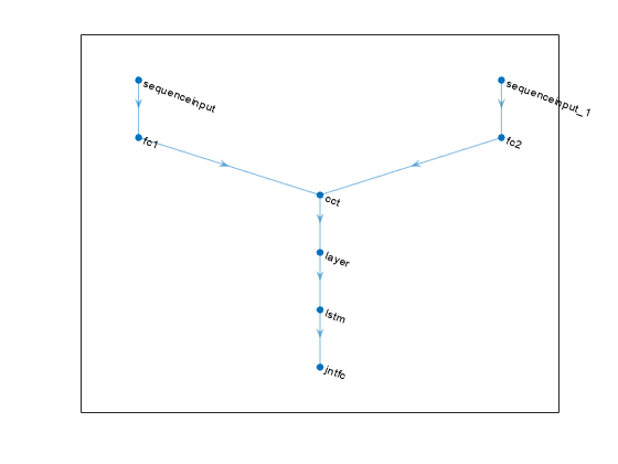
actInfo = rlFiniteSetSpec([-1 0 1]);액터 내에서 근사 모델로 사용할 심층 신경망을 만듭니다. 출력 계층은 3개 요소를 가져야 하며 각 요소는 주어진 관측값에 대해 대응하는 행동을 실행하는 가치를 표현합니다. 순환 신경망을 만들기 위해 sequenceInputLayer를 입력 계층으로 사용하고 lstmLayer를 다른 신경망 계층 중 하나로 포함합니다.
% Define paths
inPath1 = [ sequenceInputLayer(prod(obsInfo(1).Dimension))
            fullyConnectedLayer(prod(actInfo.Dimension),Name="fc1") ];

inPath2 = [ sequenceInputLayer(prod(obsInfo(2).Dimension))
            fullyConnectedLayer(prod(actInfo.Dimension),Name="fc2") ];

% Concatenate previous paths outputs along first dimension
jointPath = [ concatenationLayer(1,2,Name="cct")
              tanhLayer;
              lstmLayer(8,OutputMode="sequence");
              fullyConnectedLayer( ...
                prod(numel(actInfo.Elements)), ...
                Name="jntfc"); ];

% Add layers to network object
net = layerGraph;
net = addLayers(net,inPath1);
net = addLayers(net,inPath2);
net = addLayers(net,jointPath);

% Connect layers
net = connectLayers(net,"fc1","cct/in1");
net = connectLayers(net,"fc2","cct/in2");

% Plot network
plot(net)
% Convert to dlnetwork and display the number of weights
net = dlnetwork(net);
summary(net)
Initialized: true
Number of learnables: 386
Inputs:
1 'sequenceinput' Sequence input with 4 dimensions
2 'sequenceinput_1' Sequence input with 1 dimensions
출력 계층의 각 요소는 가능한 행동 중 하나를 실행할 확률을 나타내야 하므로, 사용자가 명시적으로 지정하지 않을 경우 softmaxLayer가 최종 출력 계층으로 자동으로 추가됩니다.
rlDiscreteCategoricalActor를 신경망, 관측값 사양 및 행동 사양 객체와 함께 사용하여 액터를 만듭니다. 신경망에 여러 개의 입력 계층이 있는 경우 obsInfo의 차원 사양에 따라 입력 계층이 자동으로 환경 관측값 채널과 연결됩니다.
actor = rlDiscreteCategoricalActor(net, obsInfo, actInfo);
각각의 가능한 행동에 대한 확률로 구성된 벡터를 반환하려면 evaluate를 사용합니다.
[prob,state] = evaluate(actor, ...
                { rand(obsInfo(1).Dimension) , ...
                  rand(obsInfo(2).Dimension) });
prob{1}
ans = 3x1 single column vector

    0.3403
    0.3114
    0.3483
분포에서 샘플링된 행동을 반환하려면 getAction을 사용합니다.
act = getAction(actor, ...
                { rand(obsInfo(1).Dimension) , ...
                  rand(obsInfo(2).Dimension) });
act{1}
ans = 1
기울기 계산 속도를 높이는 옵션을 설정합니다.
actor = accelerate(actor,true);
셀 내 각 배열에는 파라미터 그룹에 대한 출력값 합의 기울기가 들어 있습니다.
grp_batch = gradient(actor,"output-parameters", ...
                        { rand([obsInfo(1).Dimension 5 9]) , ...
                          rand([obsInfo(2).Dimension 5 9])} )
grp_batch=9×1 cell array
    {[-3.0043e-09 -4.2051e-09 -3.6952e-09 -4.0248e-09]}
    {[                                    -1.0353e-08]}
    {[                                    -7.9828e-09]}
    {[                                    -2.2359e-08]}
    {32x2 single                                      }
    {32x8 single                                      }
    {32x1 single                                      }
    { 3x8 single                                      }
    { 3x1 single                                      }
입력값 배치를 사용할 경우 gradient는 전체 입력 시퀀스(이 경우 9개 스텝)를 사용하고, 독립 배치 차원(이 경우 5)에 대한 모든 기울기가 합산됩니다. 따라서 반환되는 기울기는 항상 getLearnableParameters의 출력값과 크기가 동일합니다.
입력 인수
출력 인수
버전 내역
R2022a에 개발됨
참고 항목
함수
객체
rlValueFunction|rlQValueFunction|rlVectorQValueFunction|rlContinuousDeterministicActor|rlDiscreteCategoricalActor|rlContinuousGaussianActor|rlContinuousDeterministicTransitionFunction|rlContinuousGaussianTransitionFunction|rlContinuousDeterministicRewardFunction|rlContinuousGaussianRewardFunction|rlIsDoneFunction
You can also select a web site from the following list:
Americas
- América Latina (Español)
- Canada (English)
- United States (English)
Europe
- Belgium (English)
- Denmark (English)
- Deutschland (Deutsch)
- España (Español)
- Finland (English)
- France (Français)
- Ireland (English)
- Italia (Italiano)
- Luxembourg (English)
- Netherlands (English)
- Norway (English)
- Österreich (Deutsch)
- Portugal (English)
- Sweden (English)
- Switzerland
- United Kingdom (English)