Ground Clutter Mitigation with Moving Target Indication (MTI) Radar

This example shows the design of a moving target indication (MTI) radar to mitigate clutter and identify moving targets. For a radar system, clutter refers to the received echoes from environmental scatters other than targets, such as land, sea or rain. Clutter echoes can be many orders of magnitude larger than target echoes. An MTI radar exploits the relatively high Doppler frequencies of moving targets to suppress clutter echoes, which usually have zero or very low Doppler frequencies.

A typical MTI radar uses a high-pass filter to remove energy at low Doppler frequencies. Since the frequency response of an FIR high-pass filter is periodic, some energy at high Doppler frequencies is also removed. Targets at those high Doppler frequencies thus will not be detectable by the radar. This issue is called the blind speed problem. This example shows how to use a technique, called staggered pulse-repetition frequencies (PRFs), to address the blind speed problem.

Construct a Radar System

First, define the components of a radar system. The focus of this example is on MTI processing, so the example uses the radar system built in the example Simulating Test Signals for a Radar Receiver. You can explore the details of the radar system design through that example. Change the antenna height to 100 meters to simulate a radar mounted on top of a building. Notice that the PRF in the system is approximately 30 kHz, which corresponds to a maximum unambiguous range of 5 km.

load BasicMonostaticRadarExampleData;
sensorheight = 100;
sensormotion.InitialPosition = [0 0 sensorheight]';
prf = waveform.PRF;

Retrieve the sampling frequency, the operating frequency, and the propagation speed.

fs = waveform.SampleRate;
fc = radiator.OperatingFrequency;
wavespeed = radiator.PropagationSpeed;

In many MTI systems, especially low-end ones, the power source for the transmitter is a magnetron. Thus, the transmitter adds a random phase to each transmitted pulse. Hence, it is often necessary to restore the coherence at the receiver. Such setup is referred to as coherent on receive. In these systems, the receiver locks onto the random phases added by transmitter for each pulse. Then, the receiver removes the phase impact from the samples received within the corresponding pulse interval. Simulate a coherent on receive system by setting the transmitter and receiver as follows.

transmitter.CoherentOnTransmit = false;
transmitter.PhaseNoiseOutputPort = true;
receiver.PhaseNoiseInputPort = true;

Define Targets

Next, define two moving targets.

The first target is located at the position [1600 0 1300]. Given the radar position shown in the preceding sections, it has a range of 2 km from the radar. The velocity of the target is [100 80 0], corresponding to a radial speed of -80 m/s relative to the radar. The target has a radar cross section of 25 square meters.

The second target is located at position [2900 0 800], corresponding to a range of 3 km from the radar. Set the speed of this target to a blind speed, where the Doppler signature is aliased to the PRF. This setting prevents the MTI radar from detecting the target. Use the dop2speed function to calculate the blind speed which has a corresponding Doppler frequency equal to the PRF.

wavelength = wavespeed/fc;
blindspd = dop2speed(prf,wavelength)/2; % half to compensate round trip

tgtpos = [[1600 0 1300]',[2900 0 800]'];
tgtvel = [[100 80 0]',[-blindspd 0 0]'];
tgtmotion = phased.Platform('InitialPosition',tgtpos,'Velocity',tgtvel);

tgtrcs = [25 25];
target = phased.RadarTarget('MeanRCS',tgtrcs,'OperatingFrequency',fc);

Clutter

The clutter signal was generated using the simplest clutter model, the constant gamma model, with the gamma value set to -20 dB. Such a gamma value is typical for flatland clutter. Assume that the clutter patches exist at all ranges, and that each patch has an azimuth width of 10 degrees. Also assume that the main beam of the radar points horizontally. Note that the radar is not moving.

trgamma = surfacegamma('flatland');

clutter = constantGammaClutter('Sensor',antenna,...
    'PropagationSpeed',radiator.PropagationSpeed,...
    'OperatingFrequency',radiator.OperatingFrequency,...
    'SampleRate',waveform.SampleRate,'TransmitSignalInputPort',true,...
    'PRF',waveform.PRF,'Gamma',trgamma,'PlatformHeight',sensorheight,...
    'PlatformSpeed',0,'PlatformDirection',[0;0],...
    'MountingAngles',[0 0 0],'ClutterMaxRange',5000,...
    'ClutterAzimuthSpan',360,'PatchAzimuthSpan',10,...
    'SeedSource','Property','Seed',2011);

Simulate the Received Pulses and Matched Filter

Simulate 10 received pulses for the radar and targets defined earlier.

pulsenum = 10;

% Set the seed of the receiver to duplicate results
receiver.SeedSource = 'Property';
receiver.Seed = 2010;

rxPulse = helperMTISimulate(waveform,transmitter,receiver,...
    radiator,collector,sensormotion,...
    target,tgtmotion,clutter,pulsenum);

Then pass the received signal through a matched filter.

matchingcoeff = getMatchedFilter(waveform);
matchedfilter = phased.MatchedFilter('Coefficients',matchingcoeff);
mfiltOut = matchedfilter(rxPulse);

matchingdelay = size(matchingcoeff,1)-1;
mfiltOut = buffer(mfiltOut(matchingdelay+1:end),size(mfiltOut,1));

Perform MTI Processing Using a Three-Pulse Canceler

MTI processing uses MTI filters to remove low-frequency components in slow-time sequences. Because land clutter usually is not moving, removing low-frequency components can effectively suppress it. The three-pulse canceler is a popular and simple MTI filter. The canceler is an all-zero FIR filter with filter coefficients [1 -2 1].

h = [1 -2 1];
mtiseq = filter(h,1,mfiltOut,[],2);

Use noncoherent pulse integration to combine the slow time sequences. Exclude the first two pulses because they are in the transient period of the MTI filter.

mtiseq = pulsint(mtiseq(:,3:end));
% For comparison, also integrate the matched filter output
mfiltOut = pulsint(mfiltOut(:,3:end));

% Calculate the range for each fast time sample
fast_time_grid = (0:size(mfiltOut,1)-1)/fs;
rangeidx = wavespeed*fast_time_grid/2;

% Plot the received pulse energy again range
plot(rangeidx,pow2db(mfiltOut.^2),'r--',...
    rangeidx,pow2db(mtiseq.^2),'b-' ); grid on;
title('Fast Time Sequences Using a Uniform PRF');
xlabel('Range (m)'); ylabel('Power (dB)');
legend('Before MTI filter','After MTI filter');

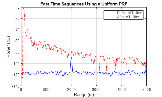
Recall that there are two targets (at 2 km and 3 km). In the case before MTI filtering, both targets are buried in clutter returns. The peak at 100 m is the direct path return from the ground right below the radar. Notice that the power is decreasing as the range increases, which is due to the signal propagation loss.

After MTI filtering, most clutter returns are removed except for the direct path peak. The noise floor is now no longer a function of range, so the noise is now receiver noise rather than clutter noise. This change shows the clutter suppression capability of the three-pulse canceler. At the 2 km range, you can see a peak representing the first target. However, there is no peak at 3 km range to represent the second target. The peak disappears because the three-pulse canceler suppresses the second target that travels at the blind speed of the canceler.

To better understand the blind speed problem, look at the frequency response of the three-pulse canceler.

f = linspace(0,prf*9,1000);
hresp = freqz(h,1,f,prf);
plot(f/1000,20*log10(abs(hresp)));
grid on; xlabel('Doppler Frequency (kHz)'); ylabel('Magnitude (dB)');
title('Frequency Response of the Three-Pulse Canceler');

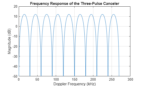
Notice the recurring nulls in the frequency response. The nulls correspond to the Doppler frequencies of the blind speeds. Targets with these Doppler frequencies are canceled by the three-pulse canceler. The plot shows that the nulls occur at integer multiples of the PRF (approximately 30kHz, 60kHz, and so on). If these nulls can be removed or pushed away from the Doppler frequency region of the radar specifications, the blind speed problem can be avoided.

Simulate the Received Pulses Using Staggered PRFs

One solution to the blind speed problem is to use nonuniform PRFs (staggered PRFs). Adjacent pulses are transmitted at different PRFs. Such a configuration pushes the lower bound of blind speeds to a higher value. To illustrate this idea, this example uses a two-staggered PRF, and then plots the frequency response of the three-pulse canceler.

Choose a second PRF at around 25kHz, which corresponds to a maximum unambiguous range of 6 km.

prf = wavespeed./(2*[6000 5000]);

% Calculate the magnitude frequency response for the three-pulse canceler
pf1 = @(f)(1-2*exp(1j*2*pi/prf(1)*f)+exp(1j*2*pi*2/prf(1)*f));
pf2 = @(f)(1-2*exp(1j*2*pi/prf(2)*f)+exp(1j*2*pi*2/prf(2)*f));
sfq = (abs(pf1(f)).^2 + abs(pf2(f)).^2)/2;

% Plot the frequency response 
hold on;
plot(f/1000,pow2db(sfq),'r--');
ylim([-50, 30]);
legend('Uniform PRF','Two-Staggered PRF');

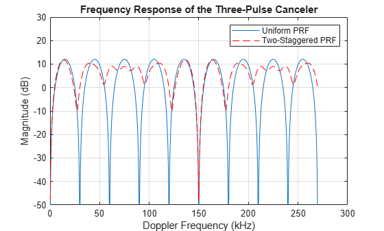
From the plot of the staggered PRFs you can see that the first blind speed corresponds to a Doppler frequency of 150 kHz, five times larger than the uniform-PRF case. Thus the target with the 30 kHz Doppler frequency will not be suppressed.

Now, simulate the reflected signals from the targets using the staggered PRFs.

% Assign the new PRF
release(waveform);
waveform.PRF = prf;

release(clutter);
clutter.PRF = prf;

% Reset noise seed
release(receiver);
receiver.Seed = 2010;

% Reset platform position
reset(sensormotion);
reset(tgtmotion);

% Simulate target return
rxPulse = helperMTISimulate(waveform,transmitter,receiver,...
    radiator,collector,sensormotion,...
    target,tgtmotion,clutter,pulsenum);

Perform MTI Processing for Staggered PRFs

Process the pulses as before by first passing them through a matched filter and then integrating the pulses noncoherently.

mfiltOut = matchedfilter(rxPulse);
% Use the same three-pulse canceler to suppress the clutter.
mtiseq = filter(h,1,mfiltOut,[],2);

% Noncoherent integration
mtiseq = pulsint(mtiseq(:,3:end));
mfiltOut = pulsint(mfiltOut(:,3:end));

% Calculate the range for each fast time sample
fast_time_grid = (0:size(mfiltOut,1)-1)/fs;
rangeidx = wavespeed*fast_time_grid/2;

% Plot the fast time sequences against range.
clf;
plot(rangeidx,pow2db(mfiltOut.^2),'r--',...
     rangeidx,pow2db(mtiseq.^2),'b-' ); grid on;
title('Fast Time Sequences Using Staggered PRFs');
xlabel('Range (m)'); ylabel('Power (dB)');
legend('Before MTI filter','After MTI filter');

The plot shows both targets are now detectable after MTI filtering, and the clutter is also removed.

Summary

With very simple operations, MTI processing can be effective at suppressing low-speed clutter. A uniform-PRF waveform will miss targets at blind speeds, but this issue can be addressed by using staggered PRFs. For clutter that has a large Doppler bandwidth, MTI performance could be poor. Such clutter can be suppressed using space-time adaptive processing. For more details, see the example Introduction to Space-Time Adaptive Processing.

References

[1] Richards, M. A. Fundamentals of Radar Signal Processing. New York: McGraw-Hill, 2005.